We left off in the last post after having discussed the Hadamard gate - our first quantum gate - and how it can be used to crate a uniform superposiiton for a single qubit. We are going to continue today by exploring other single qubit gates, discussing the underlying mathematics and, of course, testing it all out with some Q# code.

Pauli matrices in quantum mechanics 🔗

Let’s start our today’s journey by looking at the famous Pauli spin matrices, as they are central to quantum computational transformations.

In quantum mechanics, the three Pauli gates are represented by the greek letter $\sigma$, and they are shown below. They define the observable states in quantum mechanics - only the eigenstates of these matrices are in principle observable measurement values when interacting with quantum objects. The three matrices correspond to measurements done in three directions.

The presence of $i$, the imaginary number ($i=\sqrt{-1}$), in ${\sigma }_y$, is dictated by the mathematics of quantum mechanics. The state of a closed quantum system is a vector in a complex vector space and complex numbers are made up of real and imaginary components.

Pauli matrices are also of fundamental importance in quantum computing too, as they represent three of the most useful single qubit gates, and will be our main focus in this part 3 of the series.

Circuits 🔗

Similarly to classical computer science, where gates can be used to assemble circuits, in quantum computing, a sequence of quantum gates is usually referred to as a “quantum circuit”. This in turn allows visualization of the logic flow of the program at the most basic information level.

In this part 3 of the series, we are going to focus on single qubit gates only - we’ll be looking at multi qubit gates next time. In classical computing, single bit gates - at least in boolean circuits - can only exist in two variants: identity gate, which leaves the bit value intact, and a $NOT$ gate, which flips the bit value. In other words, if we input $0$ into an identity gate, $0$ would come out, and if we input $1$, then $1$ would come out. Conversely, for the $NOT$ gate, an input of $0$ produces and output of $1$ and vice versa.

In quantum computing, however, as we already mentioned in previous parts, we can come up with infinitely many single qubit gates, as there are infinitely many ways of manipulating a quantum system that the qubit represents. The reason is
quantum transformations are mathematically described by matrices - more specifically, $2^n\ast 2^n$ sized unitary matrices, where $n$ stands for the number of qubits the gate acts on, and for a single qubit case, we can construct infinite amount of unique 2 x 2 unitary matrices.

Single qubit quantum gates are often referred to as elementary quantum gates. Most general equation we can write here for quantum gates is transforming one quantum state $\psi$ to another quantum state $\phi$ using a unitary transformation:

$$U|\psi ⟩=|\phi ⟩$$

Quantum circuits can be visualized in a similar way to how classical circuits are visualized, with simple diagrams representing ordered operations on qubits. My favorite basic tool for quantum circuits is called Bono, and it can be cloned from Github and run locally; however, there are many other useful circuit building tools, one of the most popular - albeit a little overwhelming at first - being Quiirk.

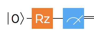
An example is shown below:

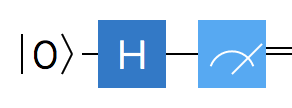
In the circuit above, we start with a single qubit in a basis state $|0⟩$, and apply the Hadamard gate that we discussed last time around - aptly marked by the H symbol. What follows is the act of measurement, which is denoted by its own measurement symbol. The line type is also of significance - a single line represents a qubit, while a double line represents a classical bit - after all, after the measurement we deal with a classical 0 or 1 value only.

Identity gate 🔗

The simplest possible quantum gate is the 2 x 2 identity gate and it semantically corresponds to the behavior of the identity gate in classical computing. Given that it is two dimensional, in linear algebra it is often denoted with $I_2$, while in quantum mechanics it is sometimes marked as $1$. In quantum computing, however, we normally just use the letter $I$ to represent the identity gate. Mathematically it can be expressed using the matrix below:

$$I=\left[\begin{array}{ccc}1& 00& 1\end{array}\right]$$

We can also say that the linear transformation behind the identity is an identity function - a function that always returns the same value as was used as its argument. We can write it in the following way:

$$I|\psi ⟩=|\psi ⟩$$

Let’s see what would happen when we apply $I$ to a qubit:

As expected, nothing really happens - when the identity gate is applied, the qubit state is left unchanged.

Pauli matrices in quantum computing 🔗

In quantum computing, when representing Pauli matrices, it is common to skip the quantum mechanical $\sigma$ notation and refer to the matrices (and thus, the quantum gates they represent) using the letters $X$, $Y$ and $Z$ only, which gives us:

As already mentioned in part 1 of this series, we are going to try to avoid imaginary and complex numbers wherever we can (it won’t always be possible) - and in this case we can simplify $Y$ and the relationship between $Y$ and ${\sigma }_y$ could be defined as:

$${\sigma }_y=-iY$$

And that’s going to be approach we will take here.

Each of the matrices can also be written using Dirac notation, as the outer product of the base vectors with their complex conjugates. This might seem somewhat confusing at first but quickly becomes very intuitive:

We shall now dive deeper into the mathematical consequences of applying each of the three Pauli gates to such a quantum system, starting with $X$.

The Pauli $X$ gate is called the bit flip gate because it ends up swapping the probability amplitudes $\alpha$ and $\beta$ with each other.

p

Since we already know that we can write the state of our qubit as the linear compination of the base vectors, with $alpha$ and $beta$ being the probability amplitudes:

$$|\phi ⟩=\alpha |0⟩+\beta |1⟩$$

we can now express the $X$ gate acting upon a qubit using simple algebra:

All of this, especially the theoretical symmetry to the classical $NOT$ gate, makes the Pauli $X$ gate one of the most important and easy to understand quantum gates.

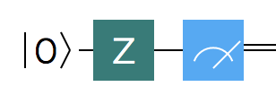
Pauli $Z$ gate flips the sign of the qubit:

In other words, we started with a state of $\alpha |0⟩+\beta |1⟩$ and ended with a state of $\alpha |0⟩-\beta |1⟩$ - the only difference being the sign. The result here may at first glance be a little confusing, especially as we already extensively discussed that the probability amplitudes can be used to obtain the actual classical probabilities of receiving a state $|0⟩$ or $|1⟩$ using the Born rule - by squaring the modulus of the amplitude $|\alpha {|}^2$ or $|\beta {|}^2$. And naturally, the change of the sign we encountered when applying the Pauli $Z$ gate has no impact on the classical probabilities. The $Z$ gate is therefore called the phase flip gate. While the phase change has no impact on probabilities of reading a classical 0 or 1 out of the qubit, it has some creative application scenarios in quantum algorithms.

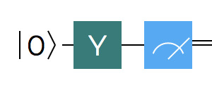
Finally, the $Y$ gate is both a bit flip gate and phase flip gate - so it swaps the amplitudes and at the same time changes the sign of the amplitude for both $|0⟩$ and $|1⟩$ (same as above, they get multiplied by $-1$).

The three Pauli gates are all its own inverses, meaning the following holds:

$$X^2=Y^2=Z^2=I$$

Pauli gates and the identity gate have fundamental meaning in quantum information theory in a sense that they can be used as building blocks to make up any other transformation. We could algebraically express any quantum computational linear transformation in the two dimensional complex vector space as a product of a complex unit and a linear combination of the three Pauli matrices and the identity matrix. It means that we can always find $\alpha$, $\beta$, $\gamma$ and $\delta$, as well as $\theta$ to represent any unitary transformation $U$:

$$U=e^{\theta i}(\alpha I+\beta X+\gamma Y+\delta Z)$$

where $\alpha$ is a real number, $\beta$, $\gamma$ and $\delta$ are complex numbers and $\theta$ is larger or equal to $0$ and smaller than $2\pi$. $e$ stands for the the Euler’s number.

Pauli gates and the identity gate in Q 🔗

We’ve spent quite some time looking at the theory, but now we are ready to go back to Q# programming. All three Pauli gates are available as functions in the $Microsoft.Quantum.Intrinsic$ namespace. These are:

• $X(qubit:Qubit)$
• $Y(qubit:Qubit)$
• $Z(qubit:Qubit)$

Identity gate is also available - mainly for completeness, but also because it is sometimes useful when an algorithm requires a no-effect action to be performed on a qubit. It is probably of no surprise to anyone that the function signature for identity is $I(qubit:Qubit)$.

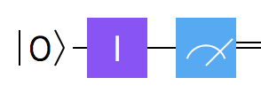
A sample Q# identity operation is shown below.

operation Identity(count : Int) : Int {

    mutable resultsTotal = 0;

    using (qubit = Qubit()) {
        for (idx in 1..count) {
            I(qubit);                
            let result = MResetZ(qubit);
            set resultsTotal += result == One ? 1 | 0;
        }

        return resultsTotal;
    }
}

The operation, similarly to the previous examples in earlier parts of this series, takes in an integer input indicating the amount of time the operation should be repeated. A single qubit is allocated within the loop, then the $I$ gate is applied and a regular measurement along the Z axis (in the computational basis) is performed. The qubit is then reset to the original state as mandated by Q# ($MResetZ$ operation guarantees the reset). We keep track of the amount of ones received by keeping a running total of the measurements. Naturally, the amount of iterations minus the amount of ones gives us the amount of zeros obtained in the measurement.

Below is the following C# driver to orchestrate this Q# operation. We will use this driver for all the snippets that come, so I will not repeat it anymore (only the invoked operation name would differ). The quantum operation would be run 1000 times to give us a better statistical result set.

class Driver
{
    static async Task Main(string[] args)
    {
        using var qsim = new QuantumSimulator();
        var iterations = 1000;
        Console.WriteLine($"Running qubit measurement {iterations} times.");
        var results = await Identity.Run(qsim, iterations);
        Console.WriteLine($"Received {results} ones.");
        Console.WriteLine($"Received {iterations - results} zeros.");
    }
}    

We should get the following output when running this program:

Running qubit measurement 1000 times.
Received 0 ones.
Received 1000 zeros.

This is of course hardly surprising. The default state of the qubit is $|0⟩$, which when measured guarantees to produce a classic bit 0. On top of that, us applying the $I$ gate doesn’t really have any effects, other than the fact that the qubit was indeed acted upon - so the 100% rate of receiving 0s is quite obvious.

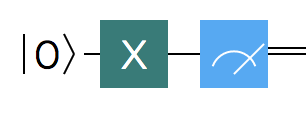
We will now turn our attention to the bit flip. The Q# code is identical to the one above, except we will use $X$ operation.

operation Bitflip(count : Int) : Int {

    mutable resultsTotal = 0;

    using (qubit = Qubit()) {
        for (idx in 1..count) {
            X(qubit);                
            let result = MResetZ(qubit);
            set resultsTotal += result == One ? 1 | 0;
        }

        return resultsTotal;
    }
}

Running this, using the same type of C# driver, would produce the following result:

Running qubit measurement 1000 times.
Received 1000 ones.
Received 0 zeros.

This is also very much in line with our expectations. The default state of the qubit is $|0⟩$, which the $X$ gate flipped to $|1⟩$ - and that, when measured, produces a bit value 1 100% percent of times.

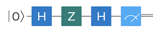
The next thing worth experimenting with is to try to chain several gates together. For example, we already made a claim - not supported by any algebraic calculation though - that the following relation holds:

$$X=HZH$$

We could verify this easily using Q#. Our operation would look as follows:

operation HZH(count : Int) : Int {
    mutable resultsTotal = 0;
    using (qubit = Qubit()) {
        for (idx in 1..count) {
            H(qubit);                
            Z(qubit);                
            H(qubit);                
            let result = MResetZ(qubit);
            set resultsTotal += result == One ? 1 | 0;
        }
        return resultsTotal;
    }
}

This code is yet again similar to the previous snippets, except this time we apply a chain of gates on the same qubit - $H-Z-H$. Running this code, with the same type of C# driver as before, produces the following result:

Running qubit measurement 1000 times.
Received 1000 ones.
Received 0 zeros.

The result is identical to running the bit flip $X$ gate, so we have really managed to experimentally verify that $X=HZH$.

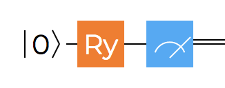
Rotation gates 🔗

As we already mentioned, there are infinitely many possibilities for constructing single qubit gates. For the purpose of this series, the 5 we already discussed - Hadamard gate $H$, Pauli gates $X$, $Y$, $Z$ and identity gate $I$ - are most important, and we will be using them repeatedly in the next parts. However, there are several other common and interesting gates, most importantly the so-called rotation gates.

$R_x$ , $R_y$ and $R_z$ are often used as part of quantum algorithms and can be utilized, for example, to prove Bell’s theorem. They are represented by the matrices below:

We mentioned that they are generializations of the Pauli gates, and looking at the matrices closely, the relation between the rotation gates and Pauli gates should become a little bit more apparent. For example, the $R_z$ gate will actually become $I$ gate when $\phi =0$, and it will become $Z$ gate when $\phi =\pi$.

Similarly to Pauli gates, all three of these rotation gates are available in Q# using the $Rx(theta:Double,qubit:Qubit)$, $Ry(theta:Double,qubit:Qubit)$ and $Rz(theta:Double,qubit:Qubit)$ functions in the $Microsoft.Quantum.Intrinsic$ namespace, where $theta$ represents the desired rotation angle.

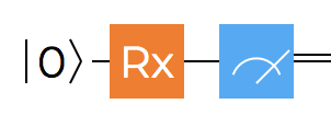
Let’s try invoking $R_x$ with a 45 degree rotation and see the effects:

operation Rx45(count : Int) : Int {
    mutable resultsTotal = 0;
    using (qubit = Qubit()) {
        for (idx in 1..count) {
            Rx(45.0, qubit);                
            let result = MResetZ(qubit);
            set resultsTotal += result == One ? 1 | 0;
        }
        return resultsTotal;
    }
}

Executing this code produces the following result:

Running qubit measurement 1000 times.
Received 251 ones.
Received 749 zeros.

So a rotation by 45 degrees along the X axis, distributes the probabilities for obtaining one or zero 0.25-0.75 - when measuring in the computational basis along the Z axis.

Summary 🔗

In this post, we discussed in depth several important quantum computing gates - Pauli gates $X$, $Y$, $Z$, as well as the identity gate $I$. In addition to that, we looked at the rotation gates too, as generalizations of the Pauli gates. In the previous post in this series, we already had a look at the Hadamard gate $H$.

All of this is still quite basic in terms of what we can do at the Q# code level, but we are slowly building up the necessary knowledge and amassing building blocks that will be extremely helpful when putting together quantum algorithms.

Equipped in this knowledge we should be are ready to have a look at multi qubit gates and the algebraic foundations behind them - which we will do in the next part. We are also going to look at one of the more bizarre quantum phenomena - entanglement. After that, we will be ready to start putting it all to good use by exploring some quantum algorithms.