Last time, we discussed the quantum teleportation protocol, which relies on the phenomenon of quantum entanglement to move an arbitrary quantum state from one qubit to another, even if they are spatially separated. Today, we shall continue exploring the scenarios enabled by entanglement, by looking at the concept called “superdense coding”. It allows communicating two classical bits of information between two parties, by moving only a single qubit between them.

Superdense coding 🔗

Superdense coding was introduced by Charles Bennett and Stephen Wiesner in their 1992 paperCommunication via one- and two-particle operators on Einstein-Podolsky-Rosen states. They realized that by applying the methodology which is effectively opposite to the decoding process applied in the teleportation scheme, they can achieve an effect of communicating two classical bits of information by sending a single qubit only

Naturally, they were still aware that because this trick relies on entanglement, quantum communication networks does not really offer twice the efficiency of data transmission of their classical counter parts - because the second qubit must have been shared between the participating parties upfront anyway.

The communication of two bits via two particles, one of which remains fixed while the other makes a round trip, is no more efficient in number of particles or number of transmissions than the obvious scheme of directly encoding each bit in one transmitted particle. Nevertheless, the EPR scheme has the advantage of allowing some of the particle transmissions to take place before the message has been decided upon, perhaps at cheaper “off’-peak” rates.

Dense coding is an interesting theoretical construct, highlighting the non-local effects of entanglement. At the same time its practical use cases are rather limited. This was highlighted by David Mermin in his book Quantum Computer Science: An Introduction:

Like dense coding, many tricks of quantum information theory, including (…) teleportation, rely on two or more people sharing entangled Qbits, prepared some time ago, carefully stored in their remote locations awaiting an occasion for their use. While the preparation of entangled Qbits (in the form of photons) and their transmission to distant places has been achieved, putting them into entanglement-preserving, local, long-term storage remains a difficult challenge.

Mathematics of superdense coding 🔗

How does it actually work?

Alice and Bob start off with a shared pair of entangled qubits. We shall refer to it as $\ket{\varphi_{ab}}$ but it is actually one of the four Bell states, the maximally entangled $\ket{\Phi^+}$.

$$\ket{\varphi_{ab}} = \frac{1}{\sqrt{2}}(\ket{00} + \ket{11}) = \ket{\Phi^+}$$

Alice encodes two bits into the pair using the reverse logic from the teleportation process:

• to encode a classical $00$, she applies the no-op $I$ transformation.
  This creates state $\frac{1}{\sqrt{2}}(\ket{00} + \ket{11}) = \ket{\Phi^+}$
• to encode a classical $01$, she applies the $X$ transformation.
  This creates state $\frac{1}{\sqrt{2}}(\ket{10} + \ket{01}) = \ket{\Psi^+}$
• to encode a classical $10$, she applies the $Z$ transformation.
  This creates state $\frac{1}{\sqrt{2}}(\ket{00} - \ket{11}) = \ket{\Phi^-}$
• to encode a classical $11$, she applies the $Y$ transformation.
  This creates state $\frac{1}{\sqrt{2}}(\ket{01} - \ket{10}) = \ket{\Psi^-}$

Next, Alice sends the qubit she transformed to Bob, so that he is in control of the entire entangled pair. At this point Bob applies the reverse Bell circuit, which we covered in the teleportation post.

Depending on the encoding initially applied by Alice, the reverse Bell circuit leads Bob to one of the following deterministic states:

$$(H \otimes I)CNOT\ket{\Phi^+} = \ket{00}$$
$$(H \otimes I)CNOT\ket{\Psi^+} = \ket{01}$$
$$(H \otimes I)CNOT\ket{\Phi^-} = \ket{10}$$
$$(H \otimes I)CNOT\ket{\Psi^-} = \ket{11}$$

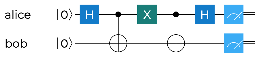
The overall schematics of it are shown on the circuit below. It illustrates the case for encoding $01$ - so using the Pauli $X$ gate, but, as we discussed moments ago, all other three would look identical, with the only difference being that particular gate.

Q# implementation of superdense coding 🔗

Let’s now shift our attention to Q# code, and try to implement the protocol using that language. Of course the protocol itself is predominantly relevant in quantum communications - where a qubit is physically transferred from one location to another. Doing it in a single Q# application process does not bring a lot of value, but it is nevertheless a useful experiment to run, to try to confirm our understanding of the foundations of quantum information theory.

We start off by allocating two qubits and entangling them, creating the Bell state $\ket{\Phi^+}$. We showed already in the earlier posts that while it is possible to manually invoke the necessary gates, we can also use the helper operation $PrepareEntangledState$ from the $Microsoft.Quantum.Preparation$ namespace.

operation TestDenseCoding(val0 : Bool, val1 : Bool) : Unit {
    using ((q0, q1) = (Qubit(), Qubit())) {
            // prepare the maximally entangled state |Φ⁺⟩ between qubits
            PrepareEntangledState([q0], [q1]);
            Encode(val0, val1, q0);
            Decode(q0, q1);
    }
}

We’d like to test the dense coding protocol for all four cases - encoding of $00$, $01$, $10$ and $11$, so it makes sense to parameterize our operation with two input bits, represented by two $Booleans$. What follows, are two operations that are not defined yet - $Encode$ and $Decode$.

The code to encode the two classical bits is shown next. Through this operation, he initial Bell state $\ket{\Phi^+}$ may stay intact or get transformed into $\ket{\Psi^+}$, $\ket{\Phi^-}$ or $\ket{\Psi^-}$.

operation Encode(val0 : Bool, val1 : Bool, qubit : Qubit) : Unit {
    mutable encoded = "";
    // if we encode 00, use Pauli I to keep |Φ⁺⟩
    if (not val0 and not val1) {
        I(qubit);
        set encoded = "00";
    }

    // if we encode 01, use Pauli X to create |Ψ⁺⟩
    if (not val0 and val1) {
        X(qubit);
        set encoded = "01";
    }

    // if we encode 10, use Pauli Z to create |Φ⁻⟩
    if (val0 and not val1) {
        Z(qubit);
        set encoded = "10";
    }

    // if we encode 11, use Pauli Y to create |Ψ⁻⟩
    if (val0 and val1) {
        Y(qubit);
        set encoded = "11";
    }
    Message("Encoded: " + encoded);
}

For the sake of tracking what we really end up encoding, we use a local mutable variable, that we can use to print out the encoded state. Finally, the decoding operation is shown below.

operation Decode(q0 : Qubit, q1 : Qubit) : Unit {
    // apply reverse Bell circuit
    CNOT(q0, q1);
    H(q0);

    // measure both qubits
    let result0 = MResetZ(q0);
    let result1 = MResetZ(q1);
    Message("Decoded: " + (result0 == One ? "1" | "0") + (result1 == One ? "1" | "0"));
}

In the end, we need to add an entry point for our application that will invoke the $TestDenseCoding$ operation with various classical bit configurations.

namespace SuperdenseCoding {

    open Microsoft.Quantum.Canon;
    open Microsoft.Quantum.Intrinsic;
    open Microsoft.Quantum.Measurement;
    open Microsoft.Quantum.Convert;
    open Microsoft.Quantum.Preparation;
    

    @EntryPoint()
    operation Start() : Unit {
    
        // encode 00
        TestDenseCoding(false, false); 
        Message("***************");
        
        // encode 01
        TestDenseCoding(false, true); 
        Message("***************");
        
        
        // encode 10
        TestDenseCoding(true, false);  
        Message("***************");
        
        // encode 11
        TestDenseCoding(true, true);  
        Message("***************");
    }
    
    // rest of the code omitted for brevity
}

Running four variants of the program, corresponding to classical bits $00$, $01$, $10$ and $11$ being encoded, and we expect the decoded output to be the same. And this is exactly what we should see as the output of our program.

Encoded: 00
Decoded: 00
***************
Encoded: 01
Decoded: 01
***************
Encoded: 10
Decoded: 10
***************
Encoded: 11
Decoded: 11
***************

Once again, we are thrilled with the result and the opportunities that quantum computing presents us with. Something that not that long ago required a complex experimental setup and some of the greatest experimental physicists on the planet, can now be achieved and verified with several lines of Q# code, and (soon) executed on quantum hardware in the cloud using Azure Quantum.

Summary 🔗

In today’s post we discussed the historical background, as well as the mathematical foundations of the superdense coding protocol. We then proceed to implement it in Q#, verifying that our algebraic reasoning was indeed correct. Similarly to teleportation, we can think of superdense coding as requiring entanglement as a resource that gets consumed when the protocol is used.

In the next parts of this series we will move towards discussing quantum security and cryptography concepts.