After a short multi-part detour into the world of quantum cryptography, in this part 12 of the series, we are going to return to some of the foundational concepts of quantum mechanics, and look at the programmatic verification of Bell’s inequality.
Where were we last time? 🔗
In part 5 we looked in detail at the phenomenon of entanglement. In that blog post, which I recommend you have a look at again before proceeding here, we introduced the famous EPR thought experiment and discussed how Bohr and others responded to this paradox. We also explored the problem of non-locality which appears to be a consequence of EPR. In fact, for Albert Einstein non-locality was the key argument proving that quantum mechanics is incomplete.
Finally, we briefly mentioned that John S. Bell, in his 1964 “On The Einstein Podolsky Rosen Paradox" formulated a test that could be used to determine whether Einstein was correct in his search for a “hidden variables” approach. And this is exactly where we will pick up in this post.
Bell’s theorem 🔗
Bell derived a mathematical inequality that is satisfied for hidden variables theories, such as those that Einstein was chasing, and that gets violated by entangled states in quantum mechanics (this was later generalized by Clauser, Horne, Shimony, and Holt). He derived his inequality for the singlet state - one of the Bell states we discussed in this series already:
$$\ket{11} \rightarrow \frac{1}{\sqrt{2}}(\ket{01} - \ket{10}) = \ket{\Psi^-}$$
Bell realized that if two pairs making up the Bell state are measured at incompatible angles $A(\theta_A)$ and $B(\theta_B)$, the quantum mechanically predicted correlation between the obtained measurements can be written as:
$$\braket{A(\theta)B(\phi)} = -cos(\theta_A - \theta_B)$$
He then followed to derive the inequality that gets violated by the predictions of quantum mechanics, but not by hidden variable theories assuming locality.
->
The original inequality that Bell derived was as follows:
$$|P(\vec{a},\vec{b}) - P(\vec{a},\vec{c})| - P(\vec{b},\vec{c}) \leq 1$$
where $P_{xy}$ refers to the average value of the product of the spins of the measured particles (qubits), $a$ and $b$ are unit vectors corresponding to the two detectors and $c$ is any other unit vector. A step-by-step derivation of the inequality is beyond our scope here, and there exist various excellent resources for that already, including Bell’s original paper and the briefly mentioned CHSH paper. John Preskill has a very accessible example using classical coins in his lecture notes, and Maccone builds upon this to provide a simple proof himself. It is also worth noting that Bell’s inequality has now been generalized to apply to a class of problems, and is available in numerous variants, hence it is being referred to in plural: inequalities.
That said, the above mentioned $\braket{A(\theta)B(\phi)}$ correlation is important, because it tells us that:
- $P(\vec{a},\vec{b}) = -cos(\theta_a - \theta_b)$
- $P(\vec{a},\vec{c}) = -cos(\theta_a - \theta_c)$
- $P(\vec{b},\vec{c}) = -cos(\theta_b - \theta_c)$
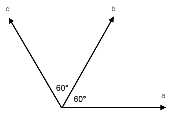
We know that cosine is a periodic function, with its values oscillating between $1$ and $-1$ so it is relatively easy to deduce from the above that there will be some angles, for which Bell’s inequalities would not be violated, and some for which the violation will be maximal. Namely, when:
- $\theta_a = 0^\circ$
- $\theta_b = \frac{\pi}{3} = 60^\circ$
- $\theta_c = \frac{\pi}{2} = 120^\circ$
Then:
- $P(\vec{a},\vec{b}) = -0.5$
- $P(\vec{a},\vec{c}) = 0.5$
- $P(\vec{b},\vec{c}) = -0.5$
And substituting these values into the inequality:
$$1.5 \nleq 1$$
Which of course is a flagrant violation of the Bell’s inequality. Bell’s theorem says:
No physical theory of local hidden variables can ever reproduce all of the predictions of quantum mechanics.
Bell’s theorem was experimentally confirmed numerous times. The first one to achieve an empirical confirmation of Bell’s inequalities was Alain Aspect, the results of which were published in 1982. Aspect wrote:
(…) our experiment yields the strongest violation of Bell’s inequalities ever achieved, and excellent agreement with quantum mechanics. Since it is a straightforward transposition of the ideal Einstein-Podolsky-Rosen-Bohm scheme, the experimental procedure is very simple, and needs no auxiliary measurements as in previous experiments with single-channel polarizers. We are thus led to the rejection of realistic local theories if we accept the assumption that there
is no bias in the detected samples: Experiments support this natural assumption.
Aspect’s experiment left two major loopholes, which have since been (mostly) closed by other experimental setups that followed. At this point is clear - with profound consequences - any local realist theory, as championed by Einstein, is wrong. This also has dramatic epistemological consequences about the very nature of reality. Elegance and Enigma dedicated a chapter to survey various physicists about the implications of Bell’s theorem. Tim Mauldin wrote there:
Assuming we can accept what we seem to see, namely, that every experiment has a unique outcome (contrary to the many-worlds view) and that the correlations between experiments performed at spacelike separation violate Bell’s inequality, then we can conclude that nature is nonlocal. That is, in some way certain events at spacelike separation are physically connected to each other. Einstein’s dream of a perfectly local physics, in which the occurrences in any small region of the spacetime depend only on what happens in that region, cannot be fulfilled. It is an open question what the implications of this fact are for the relativistic account of spacetime.
A lot of authors point to Bell’s theorem as a direct confirmation of non-locality in the fabric of nature and David Wallace even hinted at the superluminal interactions. He wrote:
The violations of Bell’s inequalities seem to tell us is that the dynamics of the microworld allows interactions that are faster than light (or slower than light but backward in time, I guess, if that really means anything). If the only interactions in the world are subluminal, Bell’s inequalities would be satisfied; they’re not, so systems can interact superluminally.
However, the view adopted in this post series, namely the reality-without-realism concept, is a lot more subtle, and more in-line with Bohr’s spirit of Copenhagen, who also advocated locality, albeit much differently than Einstein. This is nicely expressed by David Mermin, who, referring to Asher Peres’s famous statement “unperformed tests have no outcomes”, provides the following viewpoint:
So for me, nonlocality is too unsubtle a conclusion to draw from the violation of Bell inequalities. My preference is for conclusions that focus on the impropriety of seeking explanations for what might have happened but didn’t. Evolution has hard-wired us to demand such explanations, since it was crucial for our ancestors to anticipate the consequences of all possible contingencies in their (classical) struggles.
Finally, this view is corroborated by David Griffiths, who provided a very on-point and rather sharp-witted summary of the Bell’s theorem and the EPR paradox:
It is a curious twist of fate that the EPR paradox, which assumed locality in order to prove realism, led finally to the demise of locality and left the issue of realism undecided - the outcome (as Bell put it) einstein would have liked least. Most physicists today consider that if they can’t have local realism, there’s not much point in realism at all, and for this reason nonlocal hidden variable theories occupy a rather peripheral niche.
Bell’s inequalities in Q# 🔗
As we already discussed, quantum mechanics predicts that maximal violations of Bell’s inequalities will happen for the following angles:
- $\theta = \frac{\pi}{3} = 60^\circ$ angle between $\vec{a}$ and $\vec{b}$
- $\phi = \frac{\pi}{3} = 60^\circ$ angle between $\vec{b}$ and $\vec{c}$
- ($\theta + \phi) = \frac{2\pi}{3} = 120^\circ$ angle between $\vec{a}$ and $\vec{c}$
A very simple quantum computational model to validate Bell’s inequalities was summarized by Diego Garcia-Martin and German Sierra from Universidad Autonoma de Madrid in their paper Five Experimental Tests on the 5-qubit IBM Quantum Computer. We will use their approach here, with some small modifications.
We shall begin with the state $\ket{\Psi^-}$. We already know from the earlier posts, that we can obtain it from a pair of qubits in the state $\ket{11}$, running the $H$ gate on the first qubit, and then a $CNOT$ gate over both of them.
operation InitBellState(q1 : Qubit, q2: Qubit) : Unit is Adj {
    X(q1);
    X(q2);
    H(q1);
    CNOT(q1, q2);
}
We know that we need to create an experimental setup that will cater for the three different cases, corresponding to $P(\vec{a},\vec{b})$, $P(\vec{a},\vec{c})$ and $P(\vec{b},\vec{c})$. Therefore, we will define three separate Q# operations for them.
The first operation will be called $BellsInequalityAB$ and will represent $P(\vec{a},\vec{b})$
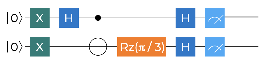
We already wrote the Q# code for the initial part of the circuit - setting up of $\ket{\Psi^-}$ state. What follows is transformation for measurement purposes. Since Q# doesn’t support measurement in an arbitrary basis, but instead only allows measurements in one of the Pauli bases, we will apply an $R_z$ rotation of $\frac{\pi}{3}$ radians. On the other hand, the circuit defines an $H$ gate followed by a standard basis $PauliZ$ measurement to achieve measurement along the X basis, but that can be expressed in the code by a single operation - measurement in $PauliX$ basis - instead. The Q# code for the circuit is shown next.
operation BellsInequalityAB() : (Bool, Bool) {
    using ((q1, q2) = (Qubit(), Qubit())) {
        InitBellState(q1, q2);
        Rz(PI() / 3.0, q2);
        return (IsResultOne(MResetX(q1)), IsResultOne(MResetX(q2)));
    }
}
The return is a tuple of two classical bits - a pair of $00$, $10$, $01$ or $11$. Pauli X basis measurement is done using the $MResetX$ built-in operation.
Our second Bell’s inequality operation will be called $BellsInequalityAC$, will correspond to $P(\vec{a},\vec{c})$ and will use $\theta = \frac{2\pi}{3} = 120^\circ$ angle between $\vec{a}$ and $\vec{c}$. The circuit is presented next.
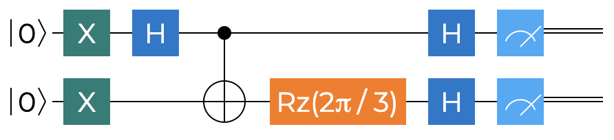
The Q# code is almost identical to the previous case - with the only exception being the wider angle.
operation BellsInequalityAC() : (Bool, Bool) {
    using ((q1, q2) = (Qubit(), Qubit())) {
        InitBellState(q1, q2);
        Rz(2.0 * PI() / 3.0, q2);
        return (IsResultOne(MResetX(q1)), IsResultOne(MResetX(q2)));
    }
}
The final circuit will allow us to measure the results for $P(\vec{b},\vec{c})$ and - as should be apparent at this point - will depend on $\theta = \frac{2\pi}{3} = 60^\circ$ angle between $\vec{b}$ and $\vec{c}$. The circuit is shown next - it is, unurprisngly, similar to the previous two variants, with the notable difference of the $R_z$ rotation gate being now applies to both qubits.
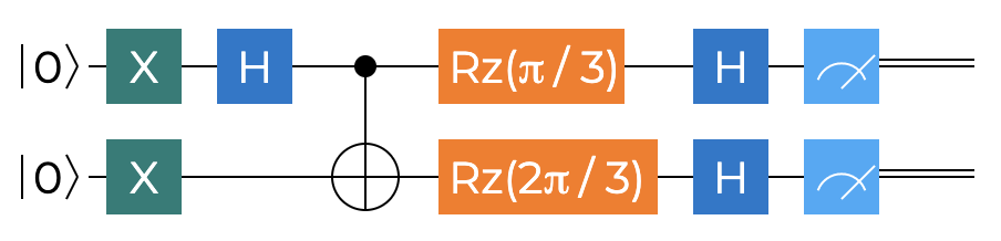
The corresponding Q# code is:
operation BellsInequalityBC() : (Bool, Bool) {
    using ((q1, q2) = (Qubit(), Qubit())) {
        InitBellState(q1, q2);
        Rz(PI() / 3.0, q1);
        Rz(2.0 * PI() / 3.0, q2);
        return (IsResultOne(MResetX(q1)), IsResultOne(MResetX(q2)));
    }
}
At this point we have all the necessary Q# operations ready - what we are still missing, is the code to orchestrate their execution, as well as some code that will output the results in an accessible format. We will, as usually, set up a small self contained Q# program for that purpose. The entry point is shown below:
@EntryPoint()
operation Main() : Unit {
        let p_ab = Run("P(a,b)", BellsInequalityAB);
        let p_ac = Run("P(a,c)", BellsInequalityAC);
        let p_bc = Run("P(b,c)", BellsInequalityBC);
        Message($"Bell's inequality |P(a,b)−P(a,c)| − P(b,c) ≤ 1, (if larger than 1, then no local hidden variable theory can reproduce QM predictions)");
        Message($"Experimental result: {DoubleAsString(AbsD(p_ab - p_ac) - p_bc)}");
}
This snippet hints at the existence of a helper $Run$ operation, which we are yet to see, that takes in two input parameters - a string identifier for the operation for visualization purposes as well as a delegate pointing to one of our three Bell inequality component operations. Such setup will allow us to reuse the output/presentation code for each of the cases. One other interesting tidbit to mention is that to make the final calculation for the Bell’s inequality, we make use of the built-in $AbsD$ function, which is part of the $Microsoft.Quantum.Math$ namespace and returns the absolute value of a double-precision floating-point number.
The $Run$ operation is shown next, completing our code.
operation Run(name : String, fn: (Unit => (Bool, Bool))) : Double {
    let runs = 4096;
    // array holding the totals of results for |00>, |01>, |10>, |11> in {runs}
    mutable results = [0, 0, 0, 0];

    for (i in 0..runs)
    {
        let (r1, r2) = fn();
        if (not r1 and not r2) { set results w/= 0 <- results[0] + 1; }
        if (not r1 and r2) { set results w/= 1 <- results[1] + 1; }
        if (r1 and not r2) { set results w/= 2 <- results[2] + 1; }
        if (r1 and r2) { set results w/= 3 <- results[3] + 1; }
    }

    let p00 = IntAsDouble(results[0]) / IntAsDouble(runs);
    let p11 = IntAsDouble(results[3]) / IntAsDouble(runs);
    let p01 = IntAsDouble(results[1]) / IntAsDouble(runs);
    let p10 = IntAsDouble(results[2]) / IntAsDouble(runs);
    let p = p00 + p11 - p01 - p10;

    Message($"|00> {p00}");
    Message($"|11> {p11}");
    Message($"|01> {p01}");
    Message($"|10> {p10}");
    Message($"{name} {p}");
    return p;
}
Ultimately, since we did all the heavy Q# parts already, this should be straight forward to read. The main purpose here is to provide a standardized way of dealing with and outputting the results of the other three operations. The sample size is fixed to 4096 runs. Since all three Bell’s inequality operations we wrote earlier return a tuple pair corresponding to the two classical bits measured, we use a 4 element mutable array to keep a running total of the obtained combinations. The compound expectation value is calculated as the sum of the probabilities of measuring $00$ or $11$ minus the probabilities of finding $01$ or $10$.
Experimental results 🔗
When running our program now, we should see results similar to the ones below.
|00> 0,1201171875
|11> 0,134033203125
|01> 0,354248046875
|10> 0,391845703125
P(a,b) -0,491943359375
|00> 0,38037109375
|11> 0,368896484375
|01> 0,135498046875
|10> 0,115478515625
P(a,c) 0,498291015625
|00> 0,119384765625
|11> 0,126708984375
|01> 0,376953125
|10> 0,377197265625
P(b,c) -0,508056640625
Bell's inequality |P(a,b)−P(a,c)| − P(b,c) ≤ 1, (if larger than 1, then no local hidden variable theory can reproduce QM predictions)
Experimental result: 1,498291015625
This is very encouraging - because it aligns perfectly with the predictions of quantum mechanics. Remember, that we expected the maximum violation to be at 1.5, because:
- $P(\vec{a},\vec{b}) = cos(60^\circ) = -0.5$
- $P(\vec{a},\vec{c}) = cos(120^\circ) = 0.5$
- $P(\vec{b},\vec{c}) = cos(60^\circ) = -0.5$
The experimentally obtained results for a trial run of 4096 repetitions are:
- $P(\vec{a},\vec{b}) = -0,491943359375$
- $P(\vec{a},\vec{c}) = 0,498291015625$
- $P(\vec{b},\vec{c}) = -0,508056640625$
This fully confirms the nonlocal nature of quantum phenomena, and excludes the possibility of local hidden variable theories. Of course at this point we are only running this in a local simulator, but very soon we’ll be able to run these in Azure on the actual quantum hardware too.
At this point it’s worth mentioning that other quantum cloud providers have already allowed similar Bell’s inequality verification to be done on their computers. The aforementioned paper from Garcia-Martin and Sierra documents their findings from running the tests on the 5-qubit IBM hardware. Their experimental results were:
- $P(\vec{a},\vec{b}) = −0.392±0.014$
- $P(\vec{a},\vec{c}) = 0.401±0.009$
- $P(\vec{b},\vec{c}) = −0.389±0.012$
This still produces the inequality violation, albeit not as large as on the Q# local simulator:
$$1.182 ± 0.020 \nleq 1$$
Their conclusion, in that case (back in 2018), was that volatility and inefficiency of the quantum circuits were still too high for scientific use cases:
Overall, the results obtained in these experiments, although moderately good in most cases, are still far from optimum.
However, the fidelity of quantum hardware has dramatically increased in the last years so I am confident that we will see real life problem solving and useful physical experiments being carried out on quantum computers in the cloud very soon. I am excited and curious to soon be able to see the results on Azure Quantum.
Summary 🔗
By proving Einstein wrong, Bell’s theorem has proven that either we need to abandon the familiar notion of local realism, or reach into non-local realist interpretative theories beyond orthodox quantum mechanics, such as Bohmian or Everrettian type. With regards to quantum computing, I continuously marvel at the fact that we can use quantum computing to experimentally verify these problems without much efforts - and doing that in Q# is a true pleasure.
This concludes part 12 of this series, last part in 2020, and we’ll continue after New Year’s! Happy Holidays!