Over the course of this series, we have developed a solid foundational understanding of quantum computing, as we learned about the basic paradigms, mathematics and various computational concepts that characterize this unique disciple. We are now well equipped to start exploring some of the most important quantum algorithms - starting with today’s part 14, which will be devoted to a simple oracle problem formulated by David Deutsch.

Historical background 🔗

The problem dates back to David Deutsch’s 1985 paper Quantum Theory, the Church-Turing Principle and the Universal Quantum Computer. In that paper, which is widely considered to have jump-started the entire research field of quantum computing, contained a reformulation of the Church-Turing thesis, which underpinned classical computation model. In 1936, an American mathematician Alonzo Church and the British mathematician Alan Turing independently of each other formulated a following hypothesis (the wording below is a rephrasing by Deutsch himself):

Every function which would naturally be regarded as computable can be computed by the universal Turing machine.

It is worth noting that the above statement is not provable - and as such it is not a theorem, but instead is taken as an axiom in computer science. The problem that Deutsch identified was with the word “naturally”, which according to him was creating mathematical ambiguity. Additionally, Deutsch pointed out that the Church-Turing conjecture is quite vague in light of the strong nature of principles in science, such as for example the law of thermodynamics. He therefore proposed a stricter version of the thesis, namely one that he referred to as ‘principle’ and which he reformulated in the following way:

Every finitely realizable physical system can be perfectly simulated by a universal model computing machine operating by finite means.

This principle was so strongly formulated that it was no longer satisfied by the Turing machine, due to the simple fact that classical computing is discrete and there exist problems e.g. classical dynamics, that are at their heart continuous. Deutsch went on to provide a description of such “perfect simulation”, which, in order to satisfy his formulation of the Church-Turing principle, led him to a conclusion that the principle requires a new computation model, namely a quantum computer:

Every existing general model of computation is effectively classical. That is, a full specification of its state at any instant is equivalent to the specification of a set of numbers, all of which are in principle measurable. Yet according to quantum theory there exist no physical systems with this property. The fact that classical physics and the classical universal Turing machine do not obey the Church-Turing principle in the strong physical form is one motivation for seeking a truly quantum model. The more urgent motivation is, of course, that classical physics is false.

The spectacular achievement of Deutsch was that he managed to not only identify the need for, but to also present the first general, fully quantum, model for computation, the so-called “Universal Quantum Computer”. Going in-depth through it - while extremely interesting from both historical and the quantum-theoretical point of view - would be out of scope for this series. However, the paper also introduced, and that would be of particular interest to us today, the first ever problem statement which a quantum computational model could be proven to solve more efficiently than its classical counterpart, at least in terms of the apparent query complexity.

Deutsch’s problem can be formulated as follows:

Given an unknown (blackbox) function that takes a single bit as an input, and produces a single bit as an ouput $f : {0,1} \rightarrow {0,1}$, determine if the function is constant or balanced.

A single bit function is constant if $f(0) = f(1)$, while it is balanced if $f(0) \neq f(1)$. A reference to a black box here stems from the approach to defining query complexity using the “oracle” concept. Using that methodology, complexity is characterized by the amount of calls to the oracle needed to solve a problem. The term black box indicates that while we provide the input values to the oracle and read its output values of the oracle, the actual implementation of it is irrelevant.

It is worth noting that in the original paper from Deutsch, the solution to the problem on a quantum computer was not deterministic and was successful only 50% of time. The solution we will discuss here is a generalized variant of the original problem that is deterministic.

Deutsch’s problem 🔗

Classically, we need two oracle calls (“function evaluations”) to solve Deutsch’s problem. For example, imagine we call $f(1)$ and receive $1$. This may mean the function is constant (always returns $1$), but it may also mean it is balanced - perhaps the output of $f(0) \neq f(1)$? To find out, we need to perform a second call $f(0)$ to find out the answer. The same logic can be extended to other possible outcomes - using classical computation model, we always need two function executions to answer the question if it is balanced or constant.

Thanks to the phenomenon of superposition, as Deutsch proved, we can use an oracle running on a quantum computer to answer this question in a single logical query. This is a key feature of quantum computing - the ability to achieve a superposition of different function evaluations is commonly called “quantum parallelism”. As Nielsen and Chuang point out:

Heuristically, and at the risk of over-simplifying, quantum parallelism allows quantum computers to evaluate a function $f(x)$ for many different values of $x$ simultaneously. In this section we explain how quantum parallelism works, and some of its limitations.

Let’s now consider how we could construct a quantum circuit that could answer this problem.

Since we use the concept of gates to express computational steps in quantum computing, an oracle will also be represented by a single quantum gate. Later on in this text, we shall nonetheless see how the internals of the oracle will look like for Deutsch’s problem use case, but for now it would be most helpful to treat it as an indivisible component. We already stated earlier in this series that any quantum gate must be unitary - which means it should be reversible. This also implies that our black box, let’s call it $U_f$ gate (there is an established convention in quantum computing to use $U$ for oracle names), must be reversible. To achieve that, the general black box must be not a single qubit but a two-qubit gate, which will look as follows:

$$U_f(\ket{x}\ket{y}) = \ket{x}\ket{y \oplus f(x)}$$

The presence of the second qubit applying the XOR logic is mandatory to guarantee reversibility - it will not be measured as part of the alogirthm though. The reversability using XOR is easy to calculate using linear algebra. Applying $U_f$ again to the output of $U_f$ leads us back to where we started from, thus fulfilling the reversibility requirement:

$$U_f(\ket{x}\ket{y \oplus f(x)}) \ = \ket{x}\ket{(y \oplus f(x)) \oplus f(x)} \ =
\ket{x}\ket{y \oplus (f(x) \oplus f(x))} \ = \ket{x}\ket{y \oplus 0} = \ket{x}\ket{y}$$

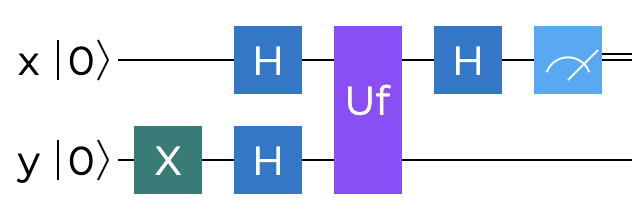
As we already know from earlier parts, we can send a qubit into a uniform superposition by using the Hadamard gate. Therefore, both $\ket{x}\ket{y}$ need to pass through the $H$ gate before they reach our $U_f$ oracle. Additionally, for reasons that will become clear in a moment, the second qubit ($\ket{y}$) needs to be flipped to the opposite ($\ket{1}$) value at the beginning of the algorithm, something that is typically achieved by the application of the $X$ gate.

Once we leave the oracle, the only measurement we need to make is on the $\ket{x}$ qubit, and we will need to run it through the $H$ gate one more time. The reason for this is that before executing the oracle, we went through a de facto change of basis process. Notice that the first application of the Hadamard gate effectively meant that we switched from the computational (Pauli Z) basis ${\ket{0}$,$\ket{1}}$ to the Hadamard (Pauli X) basis ${\ket{+}$,$\ket{-}}$. In such state, a superposition relative to the Z basis, we evaluated our oracle and afterwards, in order to measure correctly in the Z basis, we should apply $H$ gate again to undo the previous basis change. The full circuit for Deutsch’s algorithm is shown next.

In order to explore the full circuit algebraically, let’s first consider what happens to the $\ket{y}$ qubit when we pass it through the $H$ gate while keeping $\ket{x}$ intact. This will help keep the linear algebra more manageable.

$$\ket{\Psi_1} = (I \otimes H)\ket{x}\ket{1} \ = \ket{x}(\frac{1}{\sqrt{2}}(\ket{0} - \ket{1})) \ = \frac{1}{\sqrt{2}}(\ket{x}\ket{0} - \ket{x}\ket{1})$$

Continuing this line of though, let’s apply the $U_f$ oracle to such system. We should get:

$$\ket{\Psi_2} = U_f\ket{\Psi_1} \ = \ket{x}\frac{1}{\sqrt{2}}(\ket{0 \oplus f(x)} - \ket{1 \oplus f(x)})
$$

From there, we have two possibilities to go, either $f(x) = 0$ or $f(x) = 1$:

$$\ket{\Psi_2} =
\begin{cases}
\ket{x}\frac{1}{\sqrt{2}}(\ket{0} - \ket{1}) & \text{when f(x) = 0} \
\ket{x}\frac{1}{\sqrt{2}}(\ket{1} - \ket{0}) & \text{when f(x) = 1} \
\end{cases}
$$

This is exactly the point where we encounter quantum parallelism. Nielsen and Chuang provide additional context:

Naively, one might think that the state $\ket{0}\ket{f(0)} + \ket{1}\ket{f(1)}$ corresponds rather closely to a probabilistic classical computer that evaluates $f(0)$ with probability one-half, or $f(1)$ with probability one-half. The difference is that in a classical computer these two alternatives forever exclude one another; in a quantum computer it is possible for the two alternatives to interfere with one another to yield some global property of the function $f$, by using something like the Hadamard gate to recombine the different alternatives, as was done in Deutsch’s algorithm.

At this point, $\ket{\Psi_2}$ can be rewritten into a more compact form:

$$\ket{\Psi_2} = (-1)^{f(x)}\ket{x}\frac{1}{\sqrt{2}}(\ket{0} - \ket{1})
$$

What we managed to achieve here, due to the above mentioned interference, is the so called global phase kickback. The global phase now encodes the information about our function $f(x)$. We will keep this in mind as we continue our calculations. So far our math was simplified - as we kept $\ket{x}$ in a fixed state. However, for the full Deutsch’s algorithm, it’s not enough to only place the $\ket{y}$ qubit in the superposition, but we will do the same for the $\ket{x}$ qubit too - just like it was defined on the circuit above.

If we now swap $\ket{x}$ in the quantum state $\ket{\Psi_2}$ above with $H\ket{x}$, or in other words, an $\ket{x}$ in superposition, we get the following two possible outcomes:

$$\ket{\Psi_3} =
\begin{cases}
\pm\frac{1}{\sqrt{2}}(\ket{0} + \ket{1})\frac{1}{\sqrt{2}}(\ket{0} - \ket{1}) \text{ if f(0) = f(1)} \
\pm\frac{1}{\sqrt{2}}(\ket{0} - \ket{1})\frac{1}{\sqrt{2}}(\ket{0} - \ket{1}) \text{ if f(0)} \neq \text{f(1)} \
\end{cases}
$$

After going through the final Hadamard gate with the $\ket{x}$ qubit, we get it back to a definite value in the Z basis:

$$\ket{\Psi_4} =
\begin{cases}
\pm\ket{0}\frac{1}{\sqrt{2}}(\ket{0} - \ket{1}) & \text{if f(0) = f(1)} \
\pm\ket{1}\frac{1}{\sqrt{2}}(\ket{0} - \ket{1}) & \text{if f(0)} \neq \text{f(1)} \
\end{cases}
$$

At this point all that is left is to measure the $\ket{x}$ qubit. If it has the state $\ket{1}$, meaning that upon computational basis measurement the qubit will produce a classical bit $1$, then the function $f(x)$ is balanced. Otherwise, if it’s in state $\ket{0}$ and a measurement results in a classical bit $0$, it would tells us the function $f(x)$ is constant. This is a remarkable result, and one that really highlights one of the most fascinating features of quantum computing, namely quantum parallelism.

To finalize our theoretical discussions, let’s define how $U_f$ should look like for the four concrete cases defined by Deutsch’s problem. Suppose we replace our generic $f(x)$ with four specific functions $f_0$, $f_1$, $f_2$ and $f_3$, such that:

• $f_0$ is a constant $0$, namely $f(0) = f(1) = 0$
• $f_1$ is a constant $1$, namely $f(0) = f(1) = 1$
• $f_2$ is a balanced same function, namely $f(0) = 0, f(1) = 1$
• $f_3$ is a balanced flipped function, namely $f(0) = 1, f(1) = 0$

Keeping in mind the basic requirement that $U_f(\ket{x}\ket{y}) = \ket{x}\ket{y \oplus f(x)}$, the implementation of the four operations making up the $U_f$ oracle is shown below.

Do nothing for $f_0$:

$$U_{f0}(\ket{x}\ket{y}) \ = (I \otimes I)(\ket{x}\ket{y})$$

$X$ gate (bit flip) on qubit $\ket{y}$ for $f_1$:

$$U_{f1}(\ket{x}\ket{y}) \ = (I \otimes X)(\ket{x}\ket{y})$$

$CNOT$ with $\ket{x}$ as control, and $\ket{y}$ as target for $f_2$:

$$U_{f2}(\ket{x}\ket{y}) \ = CNOT(\ket{x}\ket{y})$$

$CNOT$ with $\ket{x}$ as control, and $\ket{y}$ as target, followed by $X$ (bit flip) on $\ket{y}$ for $f_3$:

$$U_{f3}(\ket{x}\ket{y}) \ = (I \otimes X)(CNOT(\ket{x}\ket{y}))$$

Deutsch’s problem in Q# 🔗

Let’s now turn our attention to implementing Deutsch’s algorithm in Q# code. The exercise should not be too challenging, as we only need to translate the above linear algebra into Q#. Just like in previous posts, we can use a standalone Q# application for running the code sample.

The first thing to do is to write the four $U_f$ oracle operations, for each of the four cases, according to how we defined them above. These operations will be used to invoke the relevant $U_f$ implementation as part of the Deutsch’s algorithm, and are shown in the snippet below.

operation OracleF0(q1 : Qubit, q2 : Qubit) : Unit is Adj {
    // constant 0
    // f(0) = f(1) = 0
}

operation OracleF1(q1 : Qubit, q2 : Qubit) : Unit is Adj  {
    // constant 1
    // f(0) = f(1) = 1
    X(q2);
}

operation OracleF2(q1 : Qubit, q2 : Qubit) : Unit is Adj  {
    // balanced same
    // f(0) = 0, f(1) = 1
    CNOT(q1, q2);
}

operation OracleF3(q1 : Qubit, q2 : Qubit) : Unit is Adj {
    // balanced opposite
    // f(0) = 1, f(1) = 0
    CNOT(q1, q2);
    X(q2);
}

Next, let’s define an orchestrator operation that can act as the implementation of the entire Deutsch’s algorithm circuit. As an input, it will accept a delegate pointing to one of the four oracle functions, and will invoke it internally, allowing us a bit more elegant approach to code and its reuse. The orchestrator function is shown next.

operation RunDeutschAlogirthm(oracle : ((Qubit, Qubit) => Unit)) : Bool {
    mutable isFunctionConstant = true;
    using ((q1, q2) = (Qubit(), Qubit())) {
        X(q2);  
        H(q1);                                    
        H(q2);

        oracle(q1, q2);                       

        H(q1);                                     

        set isFunctionConstant = MResetZ(q1) == Zero;         
        Reset(q2);       
    }
    return isFunctionConstant;
}

According to the discussion earlier, the orchestrator starts with two qubits in states $\ket{0}$. It then places one of them in state $\ket{1}$ by using the $X$ gate and then applies Hadamard gate to both of the qubits. After that, it invokes the relevant oracle operation $U_f$ that was passed to it as an argument - it will be one of the four operations we defined already. At the end, the orchestrator re-applies the $H$ gate to the qubit that will be measured, measures it and resets both of the allocated qubits. The result is then returned and tells us if the function is balanced or constant. All of this logic follows exactly our earlier outline.

Finally, the last piece of code to write is the create an entry point that will invoke the algorithm for all four oracles. Given the functions $f0$, $f1$, $f2$ and $f3$, our entry point can look like this:

@EntryPoint()
operation Main() : Unit {
    Message($"f0 is {RunDeutschAlogirthm(OracleF0) ? "constant" | "balanced"}.");
    Message($"f1 is {RunDeutschAlogirthm(OracleF1) ? "constant" | "balanced"}.");
    Message($"f2 is {RunDeutschAlogirthm(OracleF2) ? "constant" | "balanced"}.");
    Message($"f3 is {RunDeutschAlogirthm(OracleF3) ? "constant" | "balanced"}.");
}

This is everything that is needed for the entire implementation - at this point all that is left is to invoke the program, which should produce the following output, in line with our expectations.

f0 is constant.
f1 is constant.
f2 is balanced.
f3 is balanced.

Summary 🔗

While Deutsch’s problem is not really useful for any real life situations, it was a landmark achievement in terms of logically proving that quantum computers can solve a class of problems using more efficient query complexity than classical counterparts. It also demonstrated first hints of the possible quantum advantage that quantum computers can bring to the field of computing.

In the next post we shall discuss a generalization of the Deutsch’s algorithm, the so called Deutsch-Jozsa algorithm.