Mathematica 13.2 was released last month, and among the wide array of new exciting features, there is a wide set of brand new experimental astronomical computation and visualization functionalities. We will have a brief look at them in this blog post.
AstroDistance 🔗
As the name suggests, AstroDistance, returns the physical distance to or between astronomical objects (represented as entities in Mathematica), in astronomical units. For example, the current distance between Mars and Earth, in millions of kilometers, can be quickly calculated as:
UnitConvert[AstroDistance[
  Entity["Planet", "Mars"],
  { Entity["Planet", "Earth"] }
], "Gigameters"]
This produces the output which would similar to (depending of the date of course):
Quantity[122.63, "Gigameters"]
AstroDistance has several overloads as well, and in fact, the second argument is optional, and would default to your current geo-location. Since we are, well, on Planet Earth, we can therefore skip its explicit specification and simplify our earlier code to:
UnitConvert[AstroDistance[
  Entity["Planet", "Mars"]
], "Gigameters"]
Another overload, allows us to provide a date for the distance to be computed - for example, distance between Earth and Mars on 2022/12/01 can be calculated with:
UnitConvert[AstroDistance[
  Entity["Planet", "Mars"], {Entity["Planet", "Earth"],
   DateObject[{2022, 12, 01}]}], "Gigameters"]
This prints out
Quantity[81.4511, "Gigameters"]
Of course once we have the capability of providing dates, we can also easily plot the distance between the two planets over time. This can be done in a variety of ways using various Mathematica capabilities, the example with Plot is shown below (with a help of a user defined a function) - using 10 day intervals:
distanceEarthToMars[year_?NumericQ] := AstroDistance[
  Entity["Planet", "Mars"], {Entity["Planet", "Earth"],
   DateObject[{year}, CalendarType -> "GregorianYear"]}
  ]
Plot[distanceEarthToMars[year],
 {year, 2021.5, 2024},
 Filling -> Bottom,
 PlotRange -> {0, 500},
 TargetUnits -> "Gigameters",
 Exclusions -> {year ==
    DateObject[CalendarType -> "GregorianYear"]["DateList"][[1]]},
 ExclusionsStyle -> {AbsolutePointSize[10], Red}]
This provides a visualization of the changing distance between Mars and Earth from mid-2021 to the end of 2023.
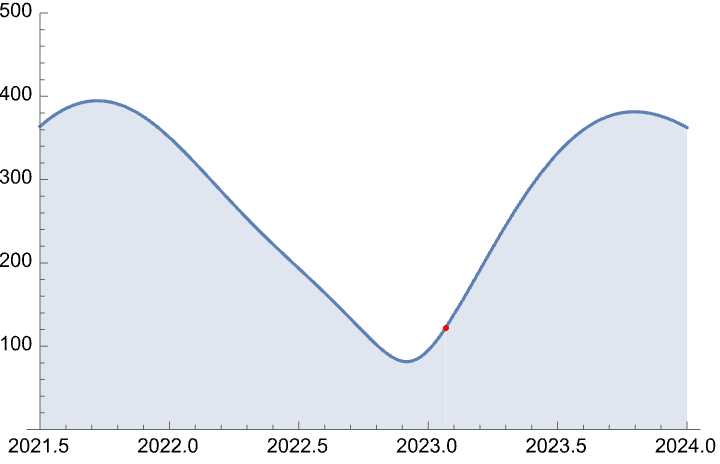
The current timestamp is marked for convenience with a red dot, using the Exclusions feature. Because of the different orbits of the planets, the distance between them constantly changes - Earth is orbiting faster than Mars, so it catches up on it, overtakes it and then races away.
In a similar fashion, we can reuse our function to find out what was the closest distance between the two planets. Here is an example of doing just that, and converting the output from the default astronomical units, to millions of kilometers:
UnitConvert[
 Quantity[
  FindMinimum[
    QuantityMagnitude[distanceEarthToMars[year]], {year, 2022,
     2024}][[1]],
  "AstronomicalUnit"],
 "Gigameters"]
This should print:
Quantity[81.4509, "Gigameters"]
AstroGrahpics 🔗
Another new feature, AstroGraphics, allows us to visualize a region of the sky, from the vantage point located anywhere in the solar system. This comes with a rich set of options such as choosing various reference frames, zoom levels, projections and more (see documenation).
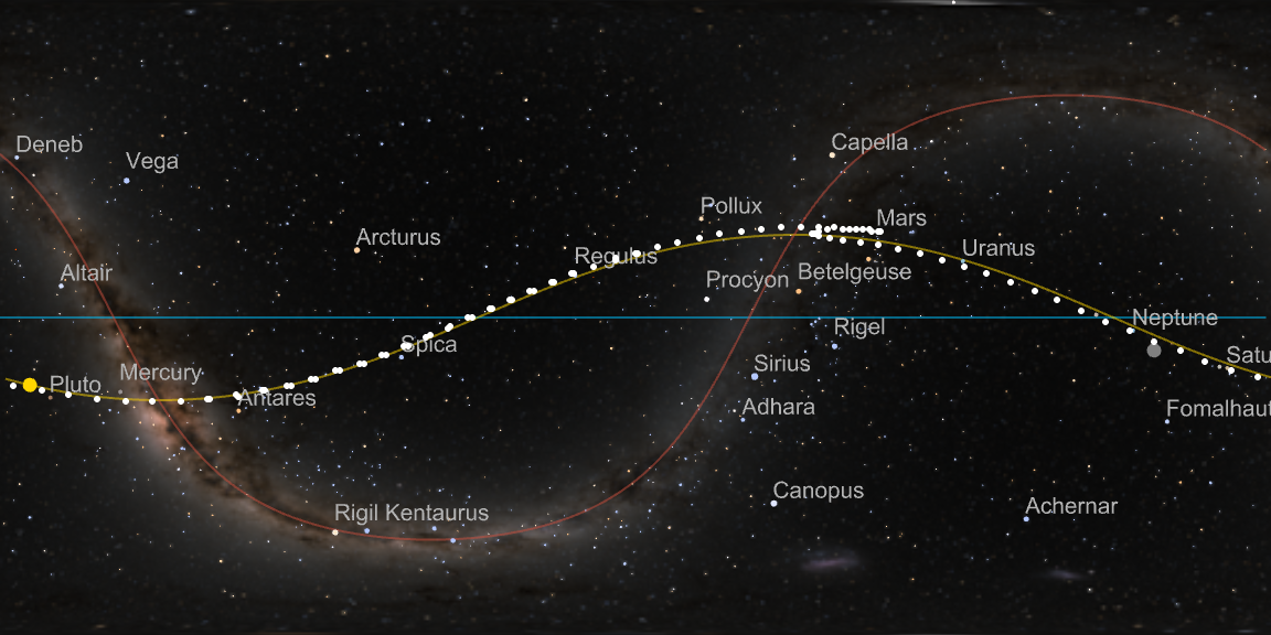
The example below draws the position of Mars on the sky between mid-2021 and end of 2023 (again at 10 day intervals), using the galactic sky backdrop and the equatorial reference frame. This visualization allows us to capture the retrograde motion of Mars that happened in that time period and just ended earlier this month.
marsPosition = AstroPosition[
     Entity["Planet", "Mars"],
     {"Equatorial", #}] & /@
   DateRange["1 July 2021", "31 December 2023", Quantity[10, "Day"]];
AstroGraphics[{White, Point[marsPosition]},
 AstroReferenceFrame -> {"Equatorial"},
 AstroBackground -> "GalacticSky"]
The output is:
Bonus: SolarSystemPlot3D 🔗
Of course the existing astro features are still there, so let’s close this post off with one that exists since Mathematica 11.3, namely SolarSystemPlot3D resource function.
We can take the same time period as we just visualized on the AstroGraphics, and use SolarSystemPlot3D to visualize the orbits of Mars and Earth during that time. This provides an interesting alternative perspective to everything we discussed so far - it shows the oscillating distance between the two planets caused by their different orbits and explains the retrograde motion as the Earth overtakes Mars.
The SolarSystemPlot3D function can be exported to the animation video as well. Several other of its features are used here to provide a nice look and feel of the generated visualization.
AnimationVideo[
 ResourceFunction["SolarSystemPlot3D"][{
   LightBlue, EdgeForm[], Sphere[Entity["Planet", "Earth"], .05],
   Orange, EdgeForm[], Sphere[Entity["Planet", "Mars"], .05]},
  date,
  Boxed -> False,
  "SunStyle" -> {Yellow, EdgeForm[],
    Lighting -> {{"Ambient", GrayLevel[.3]}, {"Directional", White,
       ImageScaled[{0, 0, 1}]}}, Sphere[{0, 0, 0}, .1]},
  Background -> Black,
  "OrbitStyle" -> Gray,
  LabelStyle -> Orange,
  "IncludeReferenceObjects" -> False,
  LabelingFunction -> Callout], {
  date, DateObject[{2021, 07, 01}], DateObject[{2023, 12, 31}],
  Quantity[7, "Days"]}, DefaultDuration -> 12]
The output of this is:
By default the animations are exported as MP4 videos, but if needed other formats can be used as well.
And this concludes a quick tour of the new (and some old) Mathematica astro features - happy exploring!