Hamiltonian simulation is the application for which quantum computers were originally proposed, and the question of how many gates it costs to simulate a given Hamiltonian to a given accuracy is one of the oldest in the field. For a long time the folklore has been that the accuracy dependence can be made logarithmic, since query-based methods such as qubitization and quantum signal processing reach an error $\epsilon$ with $O(\log(1/\epsilon))$ queries to a block encoding of the Hamiltonian.
A recent paper by Alexander Zlokapa, Richard Allen and Aram Harrow (the last of whom is a towering figure in quantum algorithms, of HHL fame), Optimal Lower Bounds for Hamiltonian Simulation (arXiv:2607.19852, 2026), argues that for many physical Hamiltonians this is not what the gate count looks like. Unless one pays for every one of the terms of the Hamiltonian, the number of gates has to grow polynomially in $1/\epsilon$.
In this post we will take the central object of that paper, a cost function that says where a Hamiltonian should be cut between a deterministic and a randomized simulation method, implement the corresponding algorithm in Q#, and measure on a 6 qubit system whether the cost function predicts what actually happens.
The Claim 🔗
Let us write the Hamiltonian as a sum of $L$ terms
$$H = \sum_{j=1}^{L} a_j h_j, \qquad \Vert h_j\Vert = 1, \qquad a_1 \geq a_2 \geq \dots \geq a_L > 0, \qquad \sum_j a_j = 1$$
so that the coefficients are sorted by size and normalized to unit total weight. The two classic product formula families sit at the opposite ends of a trade-off. A Trotter-Suzuki formula of order $2p$ has to touch every one of the $L$ terms in every step, so its gate count scales as $L \cdot t \cdot (t/\epsilon)^{1/2p}$, which is linear in the number of terms but only very weakly dependent on the accuracy. Earl Campbell’s qDRIFT, a brilliant idea from 2019, on the other hand samples terms at random with probability proportional to their weight and applies each for the same small angle. Its cost, $O(t^2/\epsilon)$, does not depend on $L$ at all (a rather remarkable property), however it pays the full price of a first-order method in $\epsilon$.
The paper’s Theorem 1 states that, for a given coefficient profile, a circuit built from two-qubit gates (single-qubit gates are free in this accounting) which simulates $e^{-iHt}$ to trace-distance error $\epsilon$ needs in general at least
$$G = \Omega\left( \min_{0 \leq K \leq L} \left[ K t + \frac{t^2 \lambda_K^2}{\epsilon} \right] \right), \qquad \lambda_K = \sum_{j > K} a_j$$
where $\lambda_K$ is the tail mass, the total weight of everything that is left after the $K$ largest terms have been taken care of. The reader will notice immediately that both classic methods are special cases of the expression inside the minimum. Choosing $K = L$ leaves no tail, so the second term vanishes and we are left with plain Trotter. Choosing $K = 0$ makes the first term vanish and the second becomes qDRIFT. The theorem says, that the best one can possibly do is to pick the $K$ that minimizes the sum. (The lower bound is a worst case over Hamiltonians with those term norms, and its hard instances are simple local classical Hamiltonians, piecewise constant in time once $t$ is large. The upper bound below holds for all of them.)
The matching upper bound is achieved by an algorithm which does exactly that. It is the elegant composite channel of Matthew Hagan and Nathan Wiebe (Composite Quantum Simulations, 2023), which Trotterizes the $K$ largest terms and qDRIFT-samples the rest.
This has two consequences whose algorithmic side we can check with a simulator. The first is that the optimal cut $K^\ast(\epsilon)$ is not a fixed property of the Hamiltonian but moves as the accuracy target shrinks (the paper’s Lemma 5 characterizes it). The second is that for the coefficient profiles the authors single out as physically relevant, namely power-law tails $a_j \propto j^{-\alpha}$ for which $\lambda_K \propto K^{1-\alpha}$, a short calculation with the objective gives a gate count growing as $\epsilon^{-1/(2\alpha-1)}$, which is a genuine polynomial no matter how clever the algorithm. The $L$ that appears in front of the query complexity of every block encoding, the authors point out, is not an artefact of a poorly optimized construction but a real cost. It cannot be removed without additional structure in the Hamiltonian. The two statements meet at $K^\ast = L$. The polynomial cost belongs to the regime in which the optimal cut is still below $L$, and once it reaches $L$ the familiar $L(t + \log(1/\epsilon))$ of a block encoding takes over, so a logarithmic dependence on the accuracy remains available to whoever pays for all $L$ terms.
The Composite Channel in Q# 🔗
The Hagan-Wiebe construction is a little more subtle than “run Trotter on the big terms, then qDRIFT on the small ones”. The two parts $A$ (the largest $K$ terms) and $B$ (the tail) are treated as the two terms of an outer product formula of order $2p$, so that the cross-commutator error between them is of high order too. Every $A$ factor of that outer formula is then implemented by an inner product formula of the same order over the terms of $A$, and every $B$ factor is implemented by a qDRIFT segment with a fixed number of samples $N_B$. The base case of the recursion is the symmetric second-order split $A(s/2)\thinspace B(s)\thinspace A(s/2)$ and the higher orders follow from Suzuki’s five-fold recursion applied to that base.
In Q# we can write this down as a short recursive operation. SuzukiStep is our own Trotter-Suzuki implementation (it follows the same recursion as TrotterArbitraryImplCA in the QDK chemistry library) and QDriftEvolve is discussed below.
operation CompositeStep(
    outerOrder : Int,
    innerOrder : Int,
    bigTerms : Pauli[][],
    bigCoeffs : Double[],
    smallTerms : Pauli[][],
    smallCoeffs : Double[],
    smallCdf : Double[],
    time : Double,
    samplesPerSegment : Int,
    qs : Qubit[]
) : Unit {
    if outerOrder == 2 {
        SuzukiStep(innerOrder, bigTerms, bigCoeffs, time / 2.0, qs);
        QDriftEvolve(smallTerms, smallCoeffs, smallCdf, time, samplesPerSegment, qs);
        SuzukiStep(innerOrder, bigTerms, bigCoeffs, time / 2.0, qs);
    } else {
        let u = SuzukiU(outerOrder);
        for slice in [u, u, 1.0 - 4.0 * u, u, u] {
            CompositeStep(
                outerOrder - 2, innerOrder,
                bigTerms, bigCoeffs, smallTerms, smallCoeffs, smallCdf,
                slice * time, samplesPerSegment, qs
            );
        }
    }
}
The qDRIFT segment samples a term index from the importance distribution $p_j = |a_j| / \lambda_B$ (a binary search over a precomputed cumulative distribution, since the tail has hundreds of terms) and applies the exponential of that term for the angle $\tau = \lambda_B \thinspace s / N_B$, carrying only the sign of the coefficient. This is the whole trick of qDRIFT. Every sampled gate has the same angle regardless of how small the term is, so the gate count depends on the total weight of the tail and not on how many terms it contains, which is what makes it the natural partner for a product formula on the few large terms.
operation QDriftEvolve(
    terms : Pauli[][],
    coeffs : Double[],
    cdf : Double[],
    time : Double,
    samples : Int,
    qs : Qubit[]
) : Unit {
    if samples > 0 {
        let tau = OneNorm(coeffs) * time / IntAsDouble(samples);
        for _ in 1..samples {
            let j = SearchCdf(cdf, DrawRandomDouble(0.0, 1.0));
            let sign = coeffs[j] >= 0.0 ? 1.0 | -1.0;
            ApplyTerm(terms[j], sign, tau, qs);
        }
    }
}
One small thing we should flag here, as it is the kind of detail that silently ruins an experiment. ApplyTerm wraps the intrinsic Exp operation, and Exp(paulis, theta, qubits) in Q# applies $e^{+i\theta P}$, not $e^{-i\theta P}$, so the physics convention $e^{-iHt}$ requires negating the angle. It is documented in the QDK source (Std/Intrinsic.qs). It is nonetheless easy to get wrong, and a test that compares a single first-order step against the same product of exponentials computed in numpy is the cheapest insurance against it.
Plain Trotter and plain qDRIFT are of course just the same code with $K = L$ and $K = 0$ respectively. We therefore end up with the whole family of algorithms the theorem talks about in a single Q# project with one integer knob.
Measuring the Error Exactly 🔗
The error metric in the theorem is the trace distance, and this is where a naive simulation goes wrong. A Trotter formula is a unitary, so one run of the Q# simulator gives the output state and the distance to the exact evolution can be computed directly. qDRIFT and the composite scheme are not unitaries but channels. Their output is the average over all random circuits that could have been sampled, and the error of the algorithm is a property of that average. Estimating it from sampled circuits is both slow and biased. With $d = 64$ amplitudes the trace norm of the sampling error of the density matrix is of the order of $\sqrt{d/M}$ after $M$ shots, so resolving $\epsilon = 10^{-2}$ would need of the order of a million shots per data point, and the bias would swamp the very quantity we are trying to measure.
Fortunately, on 6 qubits we can evaluate the channels exactly. A single qDRIFT sample is a linear map on $64 \times 64$ density matrices, and since each $U_j = e^{-i \tau P_j}$ is just $\cos\tau \thinspace I - i \sin\tau \thinspace P_j$, the map has a closed form
$$\mathcal{E}(\rho) = \cos^2\tau \thinspace \rho - i \cos\tau \sin\tau \thinspace [\hat{B}, \rho] + \sin^2\tau \sum_j p_j P_j \rho P_j, \qquad \hat{B} = B / \lambda_B$$
which in numpy is three lines, as shown in the listing below. A segment of $N_B$ samples is the $N_B$-th power of this map, the deterministic factors are unitary conjugations, and the whole composite channel is the composition of these pieces in the order in which our Q# operation applies them. We evaluate the error on one fixed entangled input state (the theorem’s $\epsilon$ is a worst case over inputs).
def apply(self, rho, tau, samples):
    c, s = np.cos(tau), np.sin(tau)
    for _ in range(samples):
        twirl = np.tensordot(self.probs, self.paulis @ rho @ self.paulis, axes=(0, 0))
        rho = c * c * rho - 1j * c * s * (self.bhat @ rho - rho @ self.bhat) + s * s * twirl
    return rho
(In the actual code the map is assembled once as a dense $4096 \times 4096$ matrix, which turned out to be about four times faster per sample, and pure qDRIFT with a million samples is handled by repeated squaring of that matrix.)
Such setup allows verifying two things, and we check both with the verify.py script in the repository before trusting any number.
The first is that the numpy mirror applies gates in exactly the order the Q# operations do. Emptying every qDRIFT segment turns the composite channel into a deterministic nest of Trotter factors, and for outer and inner orders 2 and 4 the Q# state and the numpy state agree to twelve digits or better. The second is that the Q# operations really sample from the channel we are evaluating. Running the randomized Q# operations for 96 shots and comparing the mean fidelity to the exact channel’s gives agreement within the Monte Carlo error, in every configuration tested.
5. composite channel: nested structure and sampling
  [PASS] order 2 skeleton (m=0): <Q#|rho_numpy|Q#> = 1.00000000000004
  [PASS] order 4 skeleton (m=0): <Q#|rho_numpy|Q#> = 1.00000000000083
  [PASS] order 2, r=2, m=6: Q# == exact channel: Q# 6.7971e-04 +- 2.5e-05 vs exact 6.7698e-04  (0.1 sigma)
  [PASS] order 4, r=1, m=4: Q# == exact channel: Q# 2.3729e-03 +- 1.0e-04 vs exact 2.2552e-03  (1.2 sigma)
There is one more Q# behaviour that the reader who tries to reproduce this should know about, because it produces a standard error of exactly zero and no error message. The classical random seed set with qsharp.set_classical_seed is re-applied at the start of every shot, so a multi-shot qsharp.run of a randomized operation returns the same realization over and over again. The fix is simply to run one shot per seed. The behaviour is easy to trace through the QDK source (from the Python run loop to the interpreter, which creates a fresh random number generator from the stored seed on every evaluation), and it is presumably intended for reproducibility. The seed argument of qsharp.run takes the other path and seeds shot $i$ with $\text{seed} + i$, but it gives the classical random numbers of a shot the same seed as its measurements. Nothing is measured here, so it would work too, and we keep the explicit per-shot classical seed.
The Hamiltonians and the Sweep 🔗
The paper’s motivating examples are Hamiltonians with power-law decaying coefficients, so that is what we shall use. On 6 qubits there are 693 distinct Pauli strings of weight at most 3, and we draw $L = 400$ of them at random, assign magnitudes $|a_j| \propto j^{-\alpha}$ for $\alpha \in \lbrace1.5, 2, 3\rbrace$ with random signs, normalize to $\sum_j |a_j| = 1$, and evolve for $t = 2$.
Restricting the weight keeps every term at a constant number of two-qubit gates, which is what the theorem’s gate model assumes.
We count the cost in two-qubit gates the way the resource estimator lowers them. Q#’s Exp on a weight $w$ Pauli string becomes an Rzz rotation between two CNOT ladders of $w - 2$ CNOTs each, and the estimator compiles the Rzz itself into two CNOTs around an Rz, so $2(w-1)$ CNOTs in total. The rotation counts behind that accounting are cross-checked against qsharp.logical_counts on the actual circuits (the logical counts do not list CNOTs). A native Rzz would make it $2w - 3$ for $w \geq 2$, a factor between 1.33 and 1.40 depending on the strategy, which moves the ratios below by a few percent and the fitted exponents hardly at all.
For each $\alpha$ the sweep then covers plain Trotter with orders 2 and 4 and up to 128 and 16 steps respectively, plain qDRIFT with up to $10^6$ samples, and the composite channel for every cut $K \in \lbrace 1, 2, 4, \dots, 256 \rbrace$, orders 2 and 4 with up to 16 and 4 outer steps respectively, and $N_B \in \lbrace \max(1, K/4), K, 4K \rbrace$ samples per segment. Every one of the roughly 250 configurations per $\alpha$ is evaluated exactly, which takes about 18 minutes on a laptop.
Results 🔗
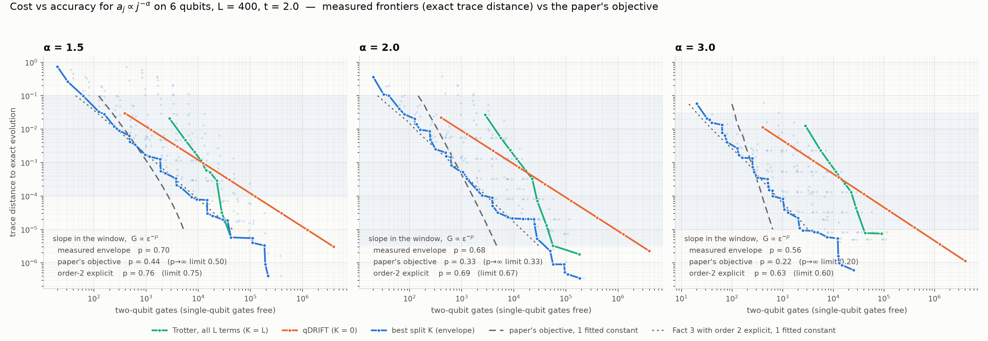
The first figure shows, for each $\alpha$, the trace distance against the number of two-qubit gates for every configuration (faint dots), with the Pareto frontier of each strategy drawn on top. The blue line is the envelope over all cuts, in other words the cost of the algorithm the theorem is actually about. The shaded band marks the window in which the paper’s own $K^\ast$ is interior ($2 \leq K^\ast \leq L/4$), which is where the asymptotic statement applies and where we do all the fits below.
Three things can be read off it, and we shall take them in turn.
The minimum over $K$ wins everywhere. Inside the window the best cut is between 15 and 49 times cheaper than plain Trotter at the coarse end of the accuracy range and between 17 and 195 times cheaper than plain qDRIFT at the fine end, depending on $\alpha$, and indeed neither endpoint is ever the cheapest option. The advantage over Trotter shrinks as $\epsilon \to 0$ at fixed $L$, since the cut creeps towards $L$. It grows with $\alpha$, since a steeper tail concentrates the weight in fewer terms, which is the regime Hagan and Wiebe describe as favourable.
The envelope follows the paper’s cost function, provided the Trotter order is kept explicit. The two grey lines are two versions of the objective, each scaled by a single fitted constant so that the shape and not the prefactor is what we compare. The dashed one is $\min_K [Kt + t^2\lambda_K^2/\epsilon]$ as written in the theorem, and it is far too steep. The dotted one is the same minimization with the Trotter term carrying its real $(t/\epsilon)^{1/2}$ factor for an order 2 formula (this is the paper’s Fact 3, Hagan and Wiebe’s cost $\Upsilon(\Upsilon L_A + N_B)$, before the order is sent to infinity), and it follows the measured envelope across the entire window, for all three values of $\alpha$.
In numbers, the exponents $G \propto \epsilon^{-p}$ we fit inside the window are
| $\alpha$ | measured envelope | paper’s objective | order 2 kept explicit |
|---|---|---|---|
| 1.5 | 0.70 | 0.44 (limit 0.50) | 0.76 (limit 0.75) |
| 2.0 | 0.68 | 0.33 (limit 0.33) | 0.69 (limit 0.67) |
| 3.0 | 0.56 | 0.22 (limit 0.20) | 0.63 (limit 0.60) |
This is not a flaw in the theorem. The Trotter term in the paper is $K t (t/\epsilon)^{o(1)}$, where the $o(1)$ is the exponent $1/2p$ of an order $2p$ formula in the limit $p \to \infty$. A real implementation has to pick a $p$, and the measured envelope here is built almost entirely from order 2 configurations (69 of the 72 envelope points inside the windows), for which that factor is $(t/\epsilon)^{1/2}$. Carrying it through the same minimization gives the exponent $(1 - 1/2p)/(2\alpha - 1) + 1/2p$, and that is, to within 0.07, what comes out of the measurement. The headline exponent $\epsilon^{-1/(2\alpha-1)}$ is what remains when the Trotter order is sent to infinity.
The second figure shows where the cut lands, with the blue step function being the $K$ of the cheapest measured configuration at each target accuracy and the two grey lines being $K^\ast(\epsilon)$ from the two versions of the objective, one with the Trotter order sent to infinity and one with it kept at 2.
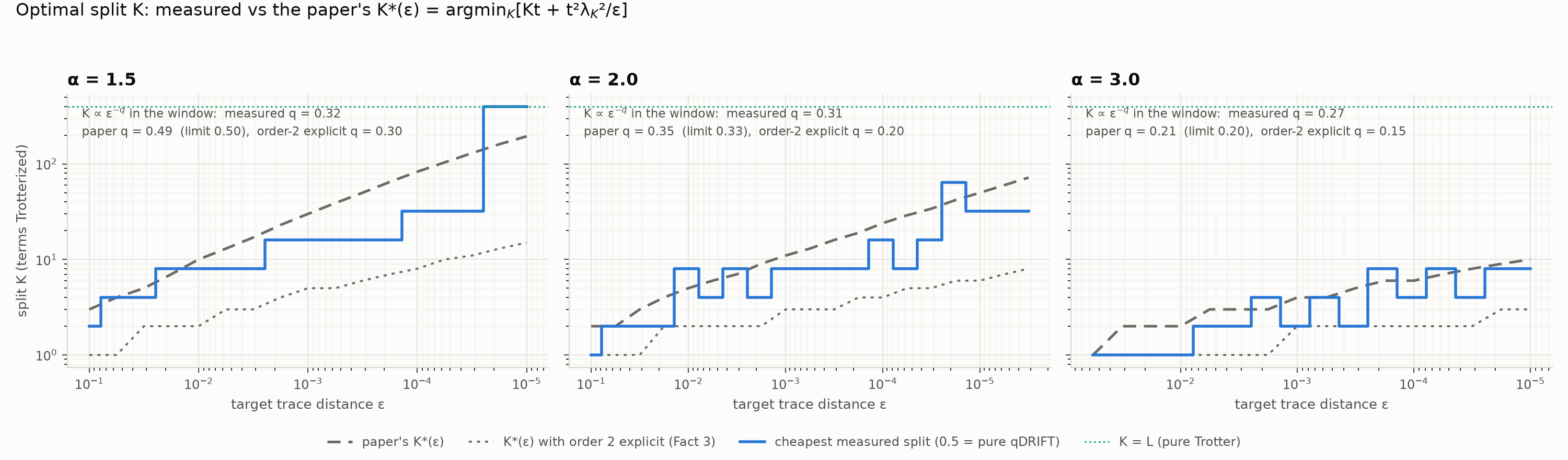
The measured cut moves as a power law, $K \propto \epsilon^{-q}$ with $q$ of 0.32, 0.31 and 0.27 for the three values of $\alpha$, and its magnitude sits between the two predictions, or one step of the power-of-two grid of cuts above the idealized one. The idealized objective over-predicts the cut and the Hagan-Wiebe upper bound constants under-predict it, which, naturally, should not be surprising, since where to cut depends on the ratio of the two prefactors that a $\Theta$ bound drops.
The exponent is another matter. The two versions of the objective predict $q$ of 0.49, 0.35 and 0.21 with the Trotter order sent to infinity, and 0.30, 0.20 and 0.15 with it kept at 2, both falling by a factor of two or more from $\alpha = 1.5$ to $\alpha = 3$, while the measured exponent falls by less than 20% and at $\alpha = 3$ is steeper than either prediction. With nine cuts spaced by factors of two, the measured $q$ is the slope of a coarse staircase, so this is no sharp test of the exponent. What the objective gets right with no fitting at all is that the cut moves as a power law of the accuracy, the order of magnitude of where it sits, and the fact that the cut is not a property of the Hamiltonian but of the Hamiltonian and the accuracy together.
Finally, since Q# comes with a resource estimator, we can translate one of these points into the currency that matters on a fault-tolerant machine. For $\alpha = 2$ and a target trace distance of $10^{-4}$, the cheapest measured configuration of each strategy, pushed through the estimator with the qubit_gate_ns_e4 qubit model and a surface code, gives
| strategy | configuration | two-qubit gates | T states | runtime |
|---|---|---|---|---|
| best cut | $K = 16$, order 2, 8 steps, $N_B = 64$ | 3 830 | 19 684 | 69 ms |
| plain Trotter | $K = 400$, order 4, 2 steps | 28 120 | 160 240 | 545 ms |
| plain qDRIFT | $N = 31\thinspace623$ | 125 575 | 664 335 | 2.6 s |
Summary 🔗
The composite qDRIFT construction is a short piece of Q#, and with an exact evaluation of the resulting channel it is possible to check, on a laptop, the achievable side of the Zlokapa-Allen-Harrow bound. The minimum over the cut is the algorithm and it beats both classic product formulas by one to two orders of magnitude in the relevant window, the cut itself moves with the accuracy as a power law, and the cost follows the paper’s objective as soon as the Trotter order hidden in its $o(1)$ is written out. What a simulation of one algorithm cannot check is the lower bound itself, the statement that nothing else does better.
The source code for this post, including the verification script, is available on GitHub.