The no-cloning theorem is usually stated as an impossibility, namely that there is no machine which takes one copy of an unknown quantum state and returns two of them. The more interesting question, posed by Reinhard Werner in 1998 in a brilliant paper on optimal cloning, is the quantitative one, that is, how well we can produce $t+1$ copies of an unknown pure state when we are given $t$ of them. The answer for arbitrary states is rather sobering, since approximate cloning turns out to need as many copies as full state tomography does, which for $n$ qubits is exponential in $n$.

Modern quantum learning theory rarely deals with arbitrary states, however. It deals with structured classes, and for some of them learning is cheap. Stabilizer states are the canonical example, since an $n$-qubit stabilizer state can be learned from $O(n)$ copies. This raises the natural question of whether the structure that makes learning easy makes cloning easier still, and a recent paper by Nikhil Bansal, Matthias Caro and Gaurav Mahajan, Cloning is as Hard as Learning for Stabilizer States (arXiv:2604.15269, 2026), answers it in the negative, since the optimal sample complexity of cloning stabilizer states turns out to be $\Theta(n)$, the same as that of learning them.

In this post we shall implement the learner in Q#, run it on the QDK’s stabilizer simulator for up to 128 qubits, and measure the mechanism behind the paper’s lower bound, which turns out to be a single fact about random vectors over $\mathbb{Z}_2$.

Stabilizer States and Bell Difference Sampling 🔗

Let us first recall what we are trying to learn. An $n$-qubit stabilizer state $|\psi\rangle$ is fixed by a group $S$ of $2^n$ commuting Pauli operators, $P|\psi\rangle = |\psi\rangle$ for every $P \in S$. Forgetting the signs of these operators, each of them is a string of $n$ single-qubit Paulis, which we can encode as a $2n$-bit vector $(a, b)$ with $Z$-part $a$ and $X$-part $b$, so that the operator is $\bigotimes_i Z^{a_i} X^{b_i}$ up to a phase. The unsigned stabilizer group is then an $n$-dimensional subspace of $\mathbb{Z}_2^{2n}$, and learning the state amounts to finding a basis of that subspace, plus $n$ signs, which is a rather more modest goal than tomography of $2^n$ amplitudes.

The tool for finding the subspace is Bell sampling, introduced for this purpose by Ashley Montanaro in 2017 and refined into Bell difference sampling by Gross, Nezami and Walter. Take two copies of the state, pair up the qubits and measure every pair in the Bell basis. The $2n$ measurement bits form a Bell label $y = (a, b)$, and for a stabilizer state that label is a uniformly random element of a coset of the unsigned stabilizer group, where the coset shift is a nuisance coming from the complex conjugation that hides inside the Bell basis, and where it is removed by taking two Bell samples and adding them modulo two. A Bell difference sample therefore costs four copies of the state and returns a uniformly random element of the unsigned stabilizer group, which is all the learner needs.

In Q# the whole procedure is a dozen lines, with the unknown state prepared by a Clifford circuit that is passed in as gate codes and which the learner never looks at.

/// Measures every pair (x[i], y[i]) in the Bell basis. The first n results are the
/// Z-part bits, the last n the X-part bits of the Bell label.
operation BellMeasure(x : Qubit[], y : Qubit[]) : Result[] {
    for i in 0..Length(x) - 1 {
        CNOT(x[i], y[i]);
        H(x[i]);
    }
    MeasureEachZ(x) + MeasureEachZ(y)
}

/// One Bell difference sample: four copies, two Bell measurements. Returns the
/// two Bell labels (2n bits each); the learner XORs them.
operation BellDifferenceSample(n : Int, gates : Int[], a : Int[], b : Int[]) : Result[] {
    use qs = Qubit[4 * n];
    for c in 0..3 {
        ApplyCircuit(gates, a, b, qs[c * n..c * n + n - 1]);
    }
    let first = BellMeasure(qs[0..n - 1], qs[n..2 * n - 1]);
    let second = BellMeasure(qs[2 * n..3 * n - 1], qs[3 * n..4 * n - 1]);
    first + second
}

Which register carries which half of the label is the kind of thing that is easy to get backwards, so the demo checks it on the state $|0\dots0\rangle$, whose stabilizer group consists of $Z$ strings only, so that every Bell difference sample of that state must have an all-zero $X$-part, and indeed it does.

Learning the State 🔗

Our learner collects Bell difference samples one at a time and keeps a row-reduced basis over $\mathbb{Z}_2$. Each new sample either lies in the span of what has been seen, in which case it is useless, or it increases the rank by one. Once the rank reaches $n$ the unsigned group is known, and the signs then cost a single further copy, since the $n$ basis elements commute, the state is an eigenstate of each of them, and measuring them jointly with Q#’s Measure returns $n$ deterministic outcomes.

operation MeasureGenerators(n : Int, gates : Int[], a : Int[], b : Int[], paulis : Pauli[][]) : Result[] {
    use qs = Qubit[n];
    ApplyCircuit(gates, a, b, qs);
    mutable out = [];
    for p in paulis {
        out += [Measure(p, qs)];
    }
    out
}

How many samples does the rank take to reach $n$? This is the question the entire paper turns on, and it has an exact answer, Lemma 5 of the paper, which is a piece of classical folklore about random vectors and which, naturally, we shall want to verify. A uniformly random vector of an $n$-dimensional space over $\mathbb{Z}_2$ lies in a given $r$-dimensional subspace with probability $2^{r-n}$, so the rank grows by one with probability $1 - 2^{r-n}$, and the probability that $k$ samples span the whole space is

$$\Pr[\text{rank} = n \text{ after } k \text{ samples}] = \prod_{i=0}^{n-1} \left(1 - 2^{,i-k}\right).$$

At $k = n$ this is $\prod_{i=1}^{n}(1 - 2^{-i})$, which decreases towards $0.2888$ and is at least $0.28$ for every $n$. At $k = n - 1$ it is, of course, exactly zero. The expected number of samples is $n + 1.607$, so the learner needs $4(n + 1.607) + 1 \approx 4n + 7.4$ copies on average.

One detail of the sign step is worth a remark, as it puzzled the present author for an afternoon. The generators the learner ends up with are almost all positive, roughly $15%$ of them carry a minus sign, whereas random elements of the same stabilizer groups are negative about half of the time. This is not a bug, however, because a row-reduced basis of a stabilizer group is, up to local Clifford gates, the canonical form of a graph state, and the canonical generators $X_i \prod_{j \sim i} Z_j$ of a graph state are all positive. The demo verifies this on an explicit graph state, and cross-checks the signs on three independent paths, the stabilizer simulator, the QDK’s full-state simulator on the same program, and a classical Aaronson-Gottesman tableau with full phase tracking.

Running It on the Stabilizer Simulator 🔗

A Bell difference sample needs $4n$ qubits, and a random stabilizer state has $2^n$ non-zero amplitudes, so the four copies together have $2^{4n}$ of them. The sparse state vector simulator we normally use from Python gives up around $n = 5$, which is no good for measuring a linear fit, and the fact that stabilizer circuits are exactly the circuits a stabilizer simulator handles in polynomial time is what rescues us. The QDK ships such a simulator, and it is reachable from Python by compiling the Q# operation to QIR under the Base profile and handing the result to run_qir with the clifford backend.

from qdk import qsharp, code
from qdk.simulation import run_qir

qsharp.init(project_root=".", target_profile=qsharp.TargetProfile.Base)

def bell_difference_samples(n, circuit, shots, seed):
    gates, a, b = circuit
    qir = qsharp.compile(code.Main.BellDifferenceSample, n, gates, a, b)
    results = run_qir(qir, shots, None, seed, "clifford")
    return np.array([learner.bell_difference(r, n) for r in results], dtype=np.uint8)

The gate codes and the Pauli strings are passed as ordinary Q# arrays and baked into the QIR, which allows compiling each random state once, at a cost of a few hundredths of a second, after which shots are essentially free. Fifty Bell difference samples of a 64-qubit state, that is a 256-qubit circuit, take about ten milliseconds. The largest states in the experiment have 128 qubits, and the whole sweep, 200 random states for each of eleven values of $n$ between 4 and 128, runs in under four minutes.

Why Cloning Cannot Be Cheaper 🔗

Now to the paper’s actual result, which is a reduction, and one that is rather hard to unsee once it has been seen.

Let us suppose we had a cloner that takes $t - 1$ copies of an unknown stabilizer state and produces $t$ copies to good accuracy. Then we could run Bell sampling on the cloned copies and obtain $t$ Bell samples from $t - 1$ copies’ worth of quantum information. In classical learning theory this is called sample amplification, a task introduced by Axelrod, Garg, Sharan and Valiant, and the paper’s first contribution is to show that for distributions which are uniform on an unknown $n$-dimensional subspace of $\mathbb{Z}_2^m$, amplifying from $n - 1$ samples to $n$ is impossible with small error, for the reason contained in the formula above, namely that from $n - 1$ samples the subspace is never determined, from $n$ samples it is determined with probability at least $0.28$, and information of that kind cannot be manufactured out of nothing.

The paper makes this quantitative with a simple distinguisher (Algorithm 1 in the paper). Given $t$ samples, run a consistent learner that outputs a uniformly random hypothesis compatible with them, and accept if the hypothesis happens to be the true subspace. On true samples the acceptance probability is the expectation of $1/N(r)$, where $r$ is the rank of the samples and $N(r)$ is the number of hypotheses consistent with $r$ independent samples. For stabilizer states the hypotheses are the Lagrangian subspaces of $\mathbb{Z}2^{2n}$ and $N(r) = \prod{i=1}^{n-r}(2^i + 1)$ of them contain a given isotropic subspace of dimension $r$. (The demo checks this by brute force at $n = 3$, where there are 135 Lagrangian subspaces in total.)

The best a sample amplifier can do is replay an element of the span it has already seen, which leaves the rank unchanged, so the distinguisher’s advantage against it is

$$\mathrm{Adv}(t) = \mathbb{E}!\left[\frac{1}{N(r_t)}\right] - \mathbb{E}!\left[\frac{1}{N(r_{t-1})}\right],$$

and Theorem 6 of the paper shows that at $t = n$ this is at least $p/2 \geq 0.14$, with $p$ the $0.28$ from above. A cloner from fewer copies would give one from more, so the bound holds for every $t \leq n$.

Two further steps carry the argument to pure stabilizer states, and both are needed. Theorem 8 shows that Bell measurement is the optimal way to extract information from copies of the mixed instance the bound is built on, so a general cloner is no better than a sample amplifier. Then a structured version of the recent random purification channel maps the mixed instances to pure stabilizer states on $4n$ qubits, which is where the factor of four in the final statement comes from. Theorem 11 then says that no cloner from fewer than $\lfloor n/4 \rfloor$ copies can reach error $0.14$ on $n$-qubit stabilizer states.

Results 🔗

Our demo measures both sides of the story from the same data, since for every random state it records the rank after each Bell difference sample, and both the learning curve and the distinguisher’s advantage follow from those records.

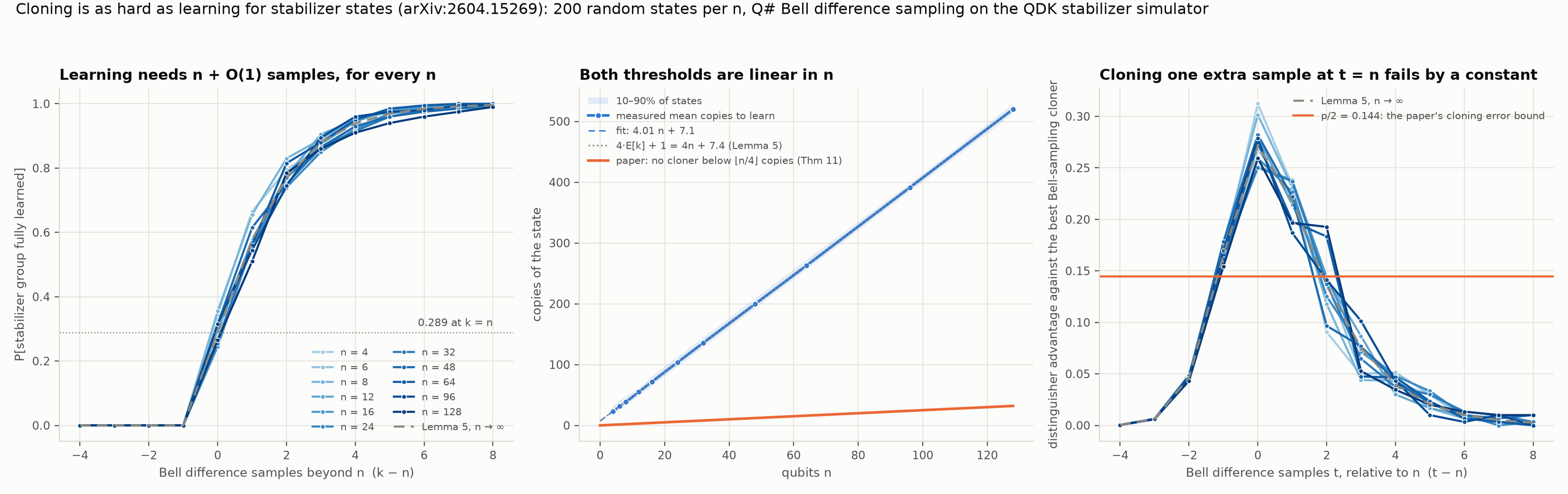
The left panel is the learning curve, the probability that the group has been fully learned as a function of the number of samples beyond $n$. All eleven values of $n$ from 4 to 128 lie on top of each other and on top of Lemma 5. At $k = n$ the measured probabilities are between $0.24$ and $0.35$ (with 200 states each the statistical error is about $0.03$), against the formula’s $0.29$.

The middle panel is the paper’s statement in one picture, in which the measured mean number of copies the learner consumes, including the one copy for signs, fits $4.005,n + 7.06$, where Lemma 5 predicts $4n + 7.43$ (the intercept sits a little low because the roughly $1%$ of states not learned within $n + 8$ samples are left out of the mean). The orange line is the paper’s impossibility threshold $n/4$, and both are straight lines, so cloning and learning are $\Theta(n)$, with a constant-factor gap of sixteen between this particular learner and the bound, and no amount of structure closes the gap between them to something sublinear.

The right panel is the proof, in the sense that the distinguisher’s advantage, computed from the measured ranks, is a bump located at $t = n$ whose height does not depend on $n$ at all. We measure it between $0.25$ and $0.31$ for every $n$, where Lemma 5 gives $0.271$ and the paper’s bound is $0.144$. Amplifying from $n - 1$ samples to $n$ is exactly one sample too early, by a constant margin that stays put as the system grows, and that constant is the whole reason cloning cannot be cheaper than learning for this class of states.

Summary 🔗

For stabilizer states, the no-cloning theorem comes with a number attached, in the sense that learning takes $n + O(1)$ Bell difference samples, cloning cannot be done from fewer than $n/4$ copies, and the obstruction is that $n - 1$ random vectors never span an $n$-dimensional space while $n$ of them do so with probability $0.29$. The QDK’s stabilizer simulator makes the whole experiment, up to 512-qubit circuits, a matter of minutes on a laptop, and we would encourage the reader to push $n$ further still.

The source code for this post, including the verification script with its nine checks, is available on GitHub.