Entanglement is fragile, and one of the more striking ways in which it is fragile was pointed out by Ting Yu and Joseph Eberly in 2004. Two qubits left to relax independently, each of them losing its excitation to its own environment, need not lose their entanglement gradually, the way the excitations themselves decay. Prepared in the state $\alpha|00\rangle + \beta|11\rangle$ with the doubly excited component the larger one, $|\beta| > |\alpha|$, they lose it completely at a finite time and it stays lost (for $|\beta| \leq |\alpha|$ it merely fades away), a phenomenon which Yu and Eberly named entanglement sudden death, and which was subsequently observed in a photonic experiment by Almeida and colleagues in 2007.
The reason it never comes back is, in fact, rather general. Once a state is separable, every further local operation keeps it separable, so local noise can only ever take entanglement away.
Magic, the other resource of quantum computation, behaves differently, and this is the subject of a recent paper by Chenfeng Cao of the Freie Universität Berlin, Sudden death of entanglement, rebirth of magic (arXiv:2605.22603, 2026). Magic (or nonstabilizerness) is the property that separates a state a Clifford circuit can prepare from one that needs a $T$ gate, and it is the resource which, when injected into an otherwise Clifford computation, makes the computation universal. The free operations of the two resource theories are simply not the same. Stabilizer operations may be entangling, and local noise channels need not preserve the stabilizer polytope, so there is no reason for magic, once lost, to stay lost.
The paper shows that for the same $n$-qubit cat states $\alpha|0^n\rangle + \beta|1^n\rangle$ under the same amplitude damping, magic dies at a finite damping strength and comes back at a larger one, while entanglement dies somewhere along the way, and that the two thresholds at which entanglement dies and magic is reborn add up to exactly one, for every $n$. Where along the way depends on $\alpha$ and $n$, since entanglement can die before the magic does, while the state is free, or only after the magic has returned.
In this post we shall build the whole trajectory in Q#, with the noise channel written as a circuit rather than as a noise model, measure the three thresholds for up to eight qubits and see where the curious identity $\gamma_e + \gamma_+ = 1$ actually comes from. Along the way we shall also extract the reborn magic onto a single qubit with nothing but parity measurements and CNOTs, which the paper proposes as a passive source of magic states.
Stabilizer states, magic and one damped qubit 🔗
Let us first fix what we mean by magic, since the word does a lot of work. The stabilizer states are the states reachable from $|0\dots0\rangle$ by Hadamard, phase and CNOT gates, and there are finitely many of them, 6 for one qubit, 60 for two, 1080 for three and 36 720 for four. A mixed state is called a stabilizer mixture (or simply free) if it is a convex combination of pure stabilizer states, and the set of all such mixtures is the stabilizer polytope $\mathcal{S}$. For a single qubit the polytope is the octahedron with the six stabilizer states $|0\rangle, |1\rangle, |\pm\rangle, |\pm i\rangle$ as vertices, that is, the set of Bloch vectors with $|x| + |y| + |z| \leq 1$.
How far a state sits outside the polytope is measured by the robustness of magic, introduced by Mark Howard and Earl Campbell in a brilliant 2017 paper on the resource theory of magic states. Any state can be written as a signed combination of stabilizer states, $\rho = \sum_j q_j \sigma_j$ with real coefficients that sum to one, and the robustness is the smallest total weight such a decomposition can have,
$$\mathcal{R}(\rho) = \min \Big\lbrace \sum_j |q_j| \hspace{0.2778em} : \hspace{0.2778em} \rho = \sum_j q_j \sigma_j, \hspace{0.2778em} \sigma_j \in \mathcal{S} \Big\rbrace.$$
For a free state $\mathcal{R} = 1$, since a convex decomposition has total weight one, and for anything else $\mathcal{R} > 1$, so $\mathcal{R} - 1$ is a faithful indicator of magic and, as Howard and Campbell showed, an upper bound on the cost of simulating the state classically. For one qubit the robustness is simply $\max(1, |x| + |y| + |z|)$.
Amplitude damping is the channel of a qubit losing its excitation, with Kraus operators
$$E_0 = |0\rangle\langle 0| + \sqrt{1-\gamma}\thinspace|1\rangle\langle 1|, \qquad E_1 = \sqrt{\gamma}\thinspace|0\rangle\langle 1|,$$
where $\gamma = 1 - e^{-\kappa t}$ is the integrated damping after time $t$ at rate $\kappa$. It leaves $|0\rangle$ alone, sends $|1\rangle$ to $|0\rangle$ with probability $\gamma$, and shrinks every coherence by $\sqrt{1-\gamma}$.
The smallest possible example of the paper’s phenomenon already lives on one qubit. Take the stabilizer state $|+\rangle$, with Bloch vector $(1, 0, 0)$, and damp it. The population of $|1\rangle$ falls from one half to $(1-\gamma)/2$, so $z$ becomes $\gamma$, while $x$ becomes $\sqrt{1-\gamma}$. The damped Bloch vector is $(\sqrt{1-\gamma}, 0, \gamma)$, and since $\sqrt{1-\gamma} + \gamma > 1$ for every $0 < \gamma < 1$, it lies outside the octahedron. Pure relaxation has manufactured magic out of a free state, which is something a Pauli channel such as depolarizing or dephasing noise could never do, since a mixture of Pauli gates maps the octahedron into itself. Being unital alone would not rule it out, because a coherent $T$ rotation is unital too and takes $|+\rangle$ out of the octahedron just as well.
The cat trajectory 🔗
The states the paper follows are the cats $|\psi_n\rangle = \alpha|0^n\rangle + \beta|1^n\rangle$ with $0 < \alpha < \beta$ and $r = \alpha/\beta$. Under amplitude damping of every qubit the state stays remarkably simple. Its only coherence is the one between $|0^n\rangle$ and $|1^n\rangle$, everything else is diagonal, and the three numbers that matter are
$$P_0 = \alpha^2 + \beta^2 \gamma^n, \qquad P_n = \beta^2 (1-\gamma)^n, \qquad c = \alpha\beta (1-\gamma)^{n/2},$$
the populations of $|0^n\rangle$ and $|1^n\rangle$ and the coherence between them. The paper’s Theorem 1 is that such a state is a stabilizer mixture exactly when
$$c \leq \min(P_0, P_n),$$
and its Theorem 4, which covers every real state of this form, gives the robustness $\mathcal{R} = 1 + 2\max\lbrace0,\thinspace c - P_0,\thinspace c - P_n\rbrace$. The necessity direction follows from the observation (Lemma 1 of the paper) that every pure stabilizer state has amplitudes of equal modulus on its support, so for any pair of basis states its coherence can never exceed the smaller of the two populations, and convex combinations inherit the bound. The sufficiency direction is an explicit decomposition into the GHZ state $(|0^n\rangle + |1^n\rangle)/\sqrt{2}$ and computational basis states. When the state has magic, the same construction with the other GHZ state, $(|0^n\rangle - |1^n\rangle)/\sqrt{2}$, entering with a negative weight gives the robustness, which we will have a use for below.
Now let us read the trajectory off these three numbers. At $\gamma = 0$ we have $c = \alpha\beta > \alpha^2 = P_0$, so the pure cat has magic, which is of course as it should be since $\alpha \neq \beta$. As $\gamma$ grows $P_0$ increases and $c$ decreases, and they cross at a value $\gamma_-$, the death of magic. The state is then free for a while, until $c$ overtakes the other population $P_n$, which happens at
$$\gamma_+ = 1 - r^{2/n},$$
after which the state has magic again all the way to $\gamma = 1$, where it finally collapses to $|0^n\rangle$. The rebirth is easy to understand from the formulas, since $c$ decays like $(1-\gamma)^{n/2}$ while $P_n$ decays like $(1-\gamma)^n$, so a coherence that is initially smaller than the population it connects ends up larger than it. Entanglement, on the other hand, dies at
$$\gamma_e = r^{2/n},$$
the point at which the negativity across every bipartition vanishes simultaneously (the partial transpose couples the coherence $c$ to a single $2 \times 2$ block whose determinant does not depend on the cut), and the state becomes fully separable. Hence
$$\gamma_e + \gamma_+ = 1$$
for every $n$, an identity which the paper connects to a symmetry of the channel itself, and which we shall take apart below.
Note that nothing here fixes the order of the three thresholds. The paper’s Corollary 1 finds three regimes, depending on $\alpha$ and $n$. Entanglement may die before the magic does ($\gamma_e < \gamma_- < \gamma_+$), in between ($\gamma_- < \gamma_e < \gamma_+$), or only after the magic has come back ($\gamma_- < \gamma_+ < \gamma_e$), in which case the rebirth happens on a state that is still entangled. For $n = 2$ the boundaries are $\alpha = 1/\sqrt{10}$ and $\alpha = 1/\sqrt{5}$, and they move to smaller $\alpha$ as $n$ grows.
Amplitude damping as a circuit 🔗
The QDK can add noise to a simulated Q# program, however only Pauli noise (bit flips, phase flips and depolarizing) and qubit loss, and its density-matrix simulator, which does accept arbitrary Kraus operators, does not run Q# code. Amplitude damping is not a Pauli channel. It is a non-unital channel, and among the phase-covariant channels the paper classifies, its non-unitality is what the whole effect rests on (a unital one with a real coherence factor never revives magic), so we shall have to build it ourselves. Fortunately every channel has a Stinespring dilation, a unitary on the system plus an environment which reproduces the channel once the environment is traced out, and for amplitude damping the canonical dilation is a two-gate circuit,
$$|0\rangle|0\rangle_E \mapsto |0\rangle|0\rangle_E, \qquad |1\rangle|0\rangle_E \mapsto \sqrt{1-\gamma}\thinspace|1\rangle|0\rangle_E + \sqrt{\gamma}\thinspace|0\rangle|1\rangle_E,$$
in which the environment qubit records whether the excitation leaked. A controlled $R_y$ rotation from the system qubit onto the environment, by the angle whose half-sine is $\sqrt{\gamma}$, followed by a CNOT back from the environment onto the system, does exactly this.
/// alpha |0^n> + beta |1^n> with beta = sqrt(1 - alpha^2).
operation PrepareCat(alpha : Double, qs : Qubit[]) : Unit {
    Ry(2.0 * ArcCos(alpha), qs[0]);
    for i in 1..Length(qs) - 1 {
        CNOT(qs[0], qs[i]);
    }
}

/// Canonical dilation of amplitude damping of strength gamma.
operation AmplitudeDamp(gamma : Double, q : Qubit, e : Qubit) : Unit {
    Controlled Ry([q], (2.0 * ArcSin(Sqrt(gamma)), e));
    CNOT(e, q);
}

operation SimDampedCat(n : Int, alpha : Double, gamma : Double) : Unit {
    use sys = Qubit[n];
    use env = Qubit[n];
    PrepareCat(alpha, sys);
    for i in 0..n - 1 {
        AmplitudeDamp(gamma, sys[i], env[i]);
    }
    DumpMachine();
    ResetAll(sys + env);
}
The SimDampedCat operation dumps the joint pure state of all $2n$ qubits, and the Python side reshapes the $4^n$ amplitudes into a $2^n \times 2^n$ matrix $M$ (the QDK orders the dump with qubit 0 as the most significant bit, so the system qubits, which were allocated first, index the rows) and takes $M M^\dagger$ for the damped system or $M^T M^*$ for the environment. Sixteen qubits at $n = 8$ take about ten milliseconds per state, so we can afford thousands of them.
Such setup has a bonus which turns out to shed light on the identity. We never throw the environment away, and the paper’s Appendix C shows that for this particular dilation the environment is left in an amplitude-damped copy of the input at the complementary strength,
$$\rho_E(\gamma) = \rho_S(1 - \gamma).$$
The matrix elements make this plain. The environment’s population of $|1\rangle$ is $\gamma\rho_{11}$, which is what damping at strength $1 - \gamma$ leaves in the excited state, and its coherence is $\sqrt{\gamma}\thinspace\rho_{01}$, which is the coherence factor of damping at strength $1 - \gamma$. The map $\gamma \leftrightarrow 1 - \gamma$ therefore exchanges the system and its environment, and on the cat it also exchanges the entanglement death condition $\beta^2\gamma^n = \alpha^2$ with the magic rebirth condition $\beta^2(1-\gamma)^n = \alpha^2$. The environment register becomes entangled at $1 - \gamma_e$, and that is exactly where the system’s magic returns.
It is worth being precise about how much of the identity this explains. On its own the reflection maps entanglement onto entanglement and magic onto magic, the system’s at $\gamma$ onto the environment’s at $1 - \gamma$. That the system’s magic comes back exactly where the environment’s entanglement appears is a second, separate fact, which the paper spells out as a mirror between the stabilizer facet $c = P_n$ of the system and the partial-transpose minor of the environment (Appendix C). The paper’s Proposition 3 states the general condition. For the whole family of phase-covariant channels it considers, the identity holds exactly when the coherence profile $S(\gamma) = \lambda(\gamma)^2/(1 - \gamma)$, with $\lambda$ the coherence factor, takes the same value at $\gamma_e$ and at $1 - \gamma_e$. Pure damping has $S \equiv 1$. Damping followed by a phase flip of fixed strength $p$ has $S \equiv (1 - 2p)^2$, so the identity survives there as well, which our verification script confirms, even though the environment of that channel is no longer a damped copy of the input.
Measuring the magic 🔗
Robustness is defined by a minimization over all stabilizer states, and for small registers we can simply do it. Enumerating the stabilizer states is a breadth-first search from $|0^n\rangle$ under the gates $H$, $S$ and CNOT on state vectors, with the global phase fixed before hashing, and the counts 60, 1080 and 36 720 confirm that nothing was missed. The minimization is then a linear program, with the density matrix’s $4^n$ real parameters as equality constraints and the signed weights split into positive and negative parts, which scipy’s HiGHS solver handles in a few seconds even at $n = 4$.
def robustness_lp(rho, states):
    N, d = states.shape
    iu = np.triu_indices(d, 1)
    feat = lambda M: np.concatenate([np.diag(M).real, M[iu].real, M[iu].imag])
    A = np.stack([feat(np.outer(s, s.conj())) for s in states], axis=1)
    res = linprog(np.ones(2 * N), A_eq=np.hstack([A, -A]), b_eq=feat(rho),
                  bounds=(0, None), method="highs")
    return res.fun
At $n = 2$, $3$ and $4$ the linear program agrees with the paper’s closed form to ten digits on both magic branches and inside the window, which is as direct a check of Theorems 1 and 4 as one could wish for. Beyond that the number of stabilizer states explodes, to 315 million at $n = 6$ and $4 \times 10^{13}$ at $n = 8$, and the linear program is out of reach. The paper’s proof, however, hands us a certificate that costs nothing.
The dual side of the theorem is a witness operator $W = \mathbb{1} + (|0^n\rangle\langle 1^n| + \mathrm{h.c.}) - 2|j^n\rangle\langle j^n|$ whose expectation lies between $-1$ and $1$ on every stabilizer state (we brute-force both bounds too, for $n \leq 4$; the lower one matters because an optimal decomposition has negative weights), so $\mathrm{Tr}(W\rho) = 1 + 2c - 2\min(P_0, P_n)$ is a lower bound on the robustness. The primal side is the explicit signed decomposition into GHZ states and basis states, which we can reconstruct numerically and whose total weight is an upper bound. The two bounds coincide at every $n$ from 5 to 8 and at every damping strength we tried, which allows using the closed form for the larger registers with a clear conscience. Entanglement, finally, needs no such care, since the negativity is just the partial transpose of the density matrix.
A dozen such checks live in the verify.py script of the repository, and the reader who wants to trust the plots below is encouraged to run it first. The two we find the most reassuring are these (the script’s equation numbers follow the HTML version of the paper on arXiv, which numbers the appendix equations on from the main text).
2. the dilation implements amplitude damping, and its environment the complementary channel
  [PASS] system == Kraus channel E_gamma (Eq. 40): max |diff| = 7.8e-16
  [PASS] environment == E_{1-gamma} of the input (Eq. 87): max |diff| = 7.8e-16
4. closed-form robustness (Theorem 4) == brute-force stabilizer-polytope LP
  [PASS] stabilizer-state counts 60, 1080, 36720: {2: 60, 3: 1080, 4: 36720}
  [PASS] LP == 1 + 2 max{0, c - P_0, c - P_n} on both magic branches and in the window: max |diff| = 8.1e-11
Death, death and rebirth 🔗
The first figure shows the trajectory. In the left panel we have two qubits with $\alpha = 0.4$, which is the paper’s own example and sits in its middle regime, with the robustness $\mathcal{R} - 1$ in blue and the negativity in red, both of which we evaluate on the exact state from Q#. Magic reaches zero at $\gamma_- = 0.324$ and stays there on the grey window, entanglement is gone for good at $\gamma_e = 0.436$, and magic returns at $\gamma_+ = 0.564$, after which it lives on a fully separable state. The window $[0.324, 0.564]$ is the one quoted in the paper, and it corresponds to $\kappa t$ between $0.39$ and $0.83$, comfortably within the $T_1$ budget of present-day hardware.
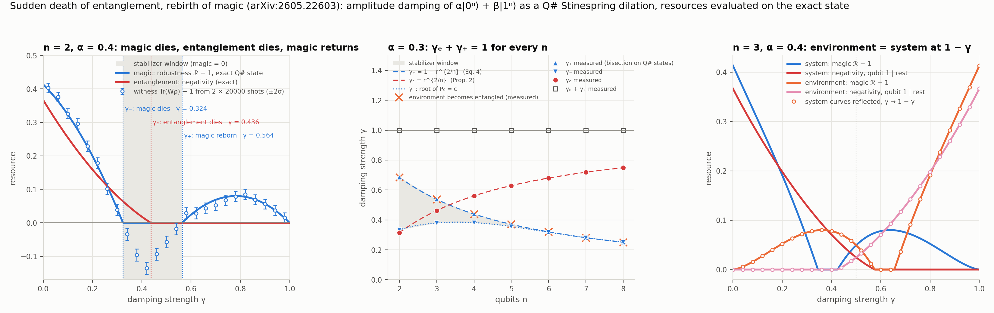
The circles in the same panel come from shots rather than from the state vector, and they show what an experiment would actually see. The witness $\mathrm{Tr}(W\rho)$ needs only two measurement settings, all qubits in the $Z$ basis (which gives $P_0$ and $P_n$) and all qubits in the $X$ basis (whose parity gives $\langle X^{\otimes n}\rangle = 2c$, since the damped cat has no other coherences), and with $20\thinspace000$ shots per setting it certifies magic at all 19 magic points at two standard deviations, and never inside the window. One should remember that this two-setting shortcut relies on the state having a single coherence, which the paper says would have to be validated on hardware by twirling or partial tomography first.
The middle panel is the identity. For $\alpha = 0.3$ and $n$ from 2 to 8 we locate the three thresholds by bisection on the simulated states, forty steps each, and plot them against the formulas. The squares are $\gamma_e + \gamma_+$ and they sit on 1 at every $n$, while the orange crosses mark the damping strength at which the environment register becomes entangled, and they sit on $\gamma_+$. The stabilizer window, the grey region between $\gamma_-$ and $\gamma_+$, closes very fast with $n$ (Proposition 1 of the paper shows it does so faster than any exponential), which the table makes rather vivid.
The order of the three thresholds, on the other hand, changes along the way, and the labels at the bottom of the panel follow it. At $n = 2$, $\alpha = 0.3$ lies below the first regime boundary $1/\sqrt{10}$ and entanglement dies before the magic does. At $n = 3$ we get the order of the left panel, and from $n = 4$ on $\gamma_+ < \gamma_e$, so the magic is reborn while the state is still entangled.
| $n$ | $\gamma_-$ | $\gamma_+$ | $\gamma_e$ | $\gamma_e + \gamma_+$ | window width | regime |
|---|---|---|---|---|---|---|
| 2 | 0.3330 | 0.6855 | 0.3145 | 1.000000 | 0.353 | I |
| 3 | 0.3797 | 0.5375 | 0.4625 | 1.000000 | 0.158 | II |
| 4 | 0.3819 | 0.4392 | 0.5608 | 1.000000 | 0.0573 | III |
| 6 | 0.3176 | 0.3200 | 0.6800 | 1.000000 | 0.00234 | III |
| 8 | 0.2511 | 0.2511 | 0.7489 | 1.000000 | 0.000030 | III |
The right panel is the mirror as curves, for three qubits. The environment’s magic and negativity (orange and pink) are the system’s curves (blue and red) reflected about $\gamma = 1/2$, to fifteen digits, and the reader can see the environment’s magic peak where the system’s is zero and vice versa. This is the environment’s side of the story. The identity itself remains a relation between the magic and the entanglement of one state, and for two qubits the paper even makes it pointwise. On the whole reborn branch the robustness excess at $\gamma$ equals $\frac{1-\gamma}{\gamma} C(1 - \gamma)$, with $C$ the concurrence (Eq. 13, which the verification script checks too).
Extracting the reborn magic 🔗
On the reborn branch the magic is, in a precise sense, nowhere in particular. Tracing out any one qubit removes the only coherence, so every proper marginal of the damped cat is diagonal and free, and for $\alpha < 1/\sqrt{1 + 2^n}$, the paper’s first two regimes, the joint state is moreover fully separable.
The paper’s Theorem 3 nonetheless shows that this nonlocal magic can be concentrated onto a single qubit with stabilizer operations alone. Measure the $n - 1$ parities $Z_i Z_{i+1}$, keep the runs in which all of them come out $+1$, which projects the state onto the span of $|0^n\rangle$ and $|1^n\rangle$ and happens with probability $P_0 + P_n \geq \alpha^2$, and decode with a cascade of CNOTs from the first qubit. The first qubit is then left in the state
$$\tilde\rho = \frac{1}{P_0 + P_n}\begin{pmatrix} P_0 & c \cr c & P_n \end{pmatrix},$$
which lies outside the octahedron exactly when the joint state lies outside the polytope, and whose robustness excess, weighted by the success probability, equals the joint state’s. Nothing is lost in expectation, and the discarded branches are all diagonal, hence free.
operation ExtractMagic(n : Int, alpha : Double, gamma : Double, basis : Int) : Result[] {
    use sys = Qubit[n];
    use env = Qubit[n];
    PrepareCat(alpha, sys);
    DampAll(gamma, sys, env);
    mutable syndrome = [];
    for i in 0..n - 2 {
        syndrome += [Measure([PauliZ, PauliZ], [sys[i], sys[i + 1]])];
    }
    for i in 1..n - 1 {
        CNOT(sys[0], sys[i]);
    }
    mutable r = Zero;
    if basis == 0 {
        r = MResetZ(sys[0]);
    } elif basis == 1 {
        r = MResetX(sys[0]);
    } else {
        r = MResetY(sys[0]);
    }
    ResetAll(sys + env);
    syndrome + [r]
}
Q#’s Measure performs the joint parity measurement without an ancilla, which a real device would need, but the protocol is otherwise exactly the paper’s. The left panel of the second figure shows the decoded qubit in the $XZ$ plane of the Bloch sphere for $\alpha = 0.2$ and $n = 2, 4, 6$, from the exact state as curves and from post-selected shots ($10\thinspace000$ per readout basis) as points with error bars. Each trajectory starts at the pure cat in the lower right, enters the octahedron (the rotated square) at $\gamma_-$, leaves it at $\gamma_+$ and ends at $|0\rangle$ on top. The dashed grey curve is the single qubit from the beginning of the post, $|+\rangle$ damped on its own, for comparison.
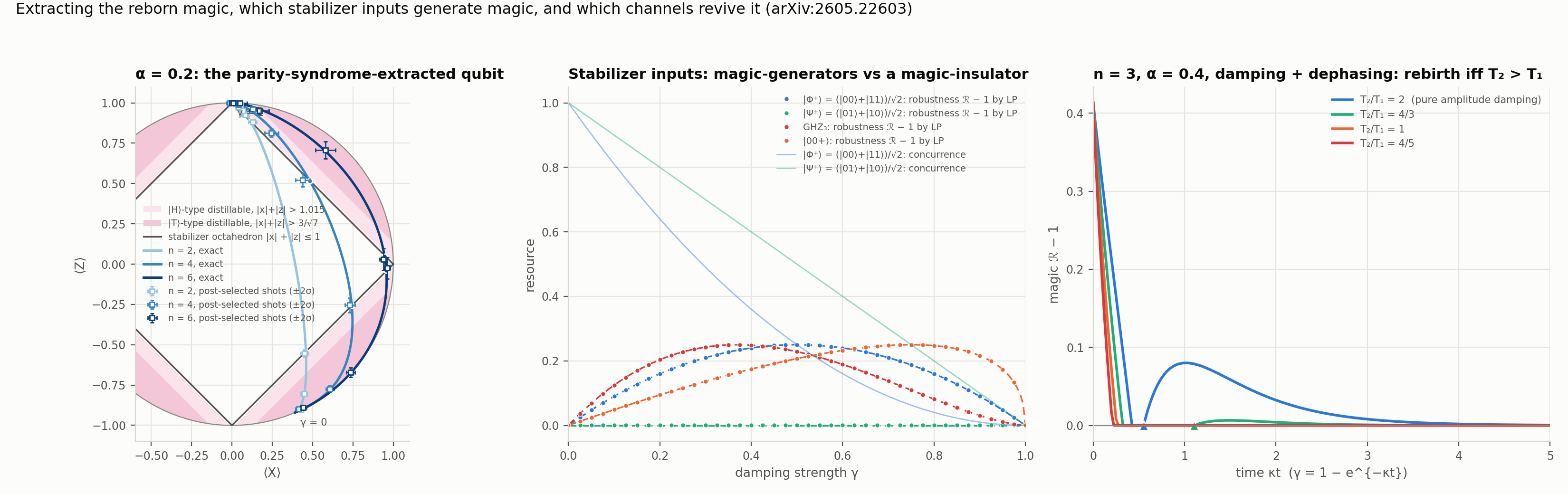
The shaded caps are the regions in which the standard Bravyi-Kitaev distillation protocols are known to work, $|x| + |z| > 1.015$ for the $|H\rangle$-type protocol and $|x| + |z| > 3/\sqrt{7} \approx 1.134$ for the $|T\rangle$-type one. The reborn branch reaches $1.02$, $1.09$ and $1.28$ for $n = 2, 4, 6$, so a longer cat pushes the extracted qubit deeper into distillable territory, and at six qubits it clears the stricter threshold.
Two remarks keep this in proportion. First, the damped $|+\rangle$ reaches $x + z = 5/4$ at $\gamma = 3/4$, which is already inside the $|T\rangle$-type window, so the point of the cat is not the onset of distillability. The paper’s case for the collective route is the yield and the quality it reaches, with the reborn branch approaching the pure $|H\rangle$ state, $x + |z| \to \sqrt{2}$, as $n$ grows. Second, $\alpha = 0.2$ enters the third regime from $n = 5$ on, so the best $n = 6$ points, around $\gamma \approx 0.52$ against $\gamma_e \approx 0.59$, are extracted from a state that is still entangled. The separable magic of the previous section is what the $n = 2$ and $n = 4$ trajectories harvest.
The paper also works out the yield, the expected robustness excess per register, and finds it can never exceed $\alpha^2/2$, which for $\alpha = 0.2$ is $0.02$, and indeed the best we find at the sampled points is $0.0200$.
Which free states generate magic, and which channels revive it 🔗
Two further results of the paper round the picture off, and both take a few lines to check once the machinery is in place.
The first is a classification. Amplitude damping is not Clifford-covariant, so two stabilizer states that a local Clifford gate maps onto each other can respond to it in opposite ways. On a single qubit $|0\rangle$ and $|+\rangle$, related by a Hadamard, already do, and the two-qubit Bell states are the smallest example in which both states are entangled. Under damping $|\Phi^+\rangle = (|00\rangle + |11\rangle)/\sqrt{2}$ leaves the polytope immediately, with robustness excess $\gamma(1 - \gamma)$, while $|\Psi^+\rangle = (|01\rangle + |10\rangle)/\sqrt{2}$ stays free for every $\gamma$, even though their entanglement decays smoothly in both cases.
Proposition 5 of the paper explains this by the computational-basis support alone. A pure stabilizer state is an insulator, immune to damping, exactly when every string in its support has the same Hamming weight, which is true of $\lbrace01, 10\rbrace$ and false of $\lbrace00, 11\rbrace$, and it is a generator otherwise. Insulators are rare, 8 of the 60 two-qubit stabilizer states, 32 of 1080, 220 of 36 720, numbers our enumeration reproduces. The middle panel shows the linear-program robustness of the two Bell states, of the three-qubit GHZ state and of the product state $|00+\rangle$ under damping, all on top of the paper’s closed profiles.
The second is a condition on the channel. Real hardware does not only relax, it dephases too, and dephasing shrinks the coherence $c$ without touching the populations, which can only hurt the rebirth. The paper’s Theorem 2 gives the answer for relaxation at rate $1/T_1$ with concurrent pure dephasing. The coherence factor becomes $q^a$ with $q = e^{-t/T_1}$ and $a = 1/2 + \Gamma_\phi T_1$, and magic is reborn if and only if $a < 1$, which in the usual language is $T_2 > T_1$.
In the demo we compose the damping dilation with a phase-flip dilation of the strength that reproduces this coherence factor at each time, and the right panel shows the result for three qubits with $\alpha = 0.4$. With $T_2 = 2T_1$ (no dephasing at all) and $T_2 = 4T_1/3$ the magic comes back, at $\kappa t = 0.5527$ and $1.1055$, which are the paper’s $q_+ = r^{1/((1-a)n)}$ to five digits, while at $T_2 = T_1$ and below it dies and stays dead. Rebirth, in other words, is a feature of cold and relaxation-dominated environments, and the paper notes that transmons already reach $T_2$ comparable to or above $T_1$, with dynamical decoupling pushing it towards the ceiling of $2T_1$.
Summary 🔗
Local Markovian noise can only destroy entanglement, but it can create magic, and the amplitude-damped cat does both, with the death of entanglement and the rebirth of magic reflected about $\gamma = 1/2$ for every register size, in whichever order the three thresholds come. The reflection has a natural reading on the environment register of the channel’s Stinespring dilation, which writing the channel as a circuit in Q# makes visible, although the coincidence of magic and entanglement behind it comes from the channel’s coherence profile rather than from the dilation alone. The reborn magic is nonlocal but can be harvested by parity measurements, and it survives dephasing precisely when $T_2 > T_1$.
The source code for this post, including the verification script and the stabilizer-polytope linear program, is available on GitHub.